1-way ANOVA contradicts nested ANOVA

Question

I have a response "rate" that has two factors "variety" and "strain" as possible covariates. I am trying to figure out if the different levels of "strain" have the same effect on "rate".

When I run one way ANOVA: anova<-aov(rate~strain, data=table), I get the following table:

             Df  Sum Sq   Mean Sq      F value Pr(>F)  
strain       6   0.001867 0.0003112    2.25    0.0675 .
Residuals   28   0.003872 0.0001383  

According to this the different levels of "strain" have the same effect on "rate" at a 5% level.

Now if I run the following model :anova<-aov(rate~strain+variety, data=table), I get the following table:

             Df    Sum Sq    Mean Sq     F value   Pr(>F)    
strain       6     0.0018670 0.0003112   8.618     4.70e-05 ***
variety      4     0.0030056 0.0007514  20.810     1.63e-07 ***
Residuals   24     0.0008666 0.0000361    

This is telling me I should definitely include strain in my model, which means the different levels of "strain" have different effects on "rate".

Why do they not agree? Which should I believe? Thank you in advance!

PS: In case it is important to know where my data is coming from, here it is: read.table("http://users.stat.ufl.edu/~winner/data/apple1.dat", header=FALSE)

Answer 1

We read in your data and reproduce the results:

df = read.table("http://users.stat.ufl.edu/~winner/data/apple1.dat",header=FALSE)
colnames(df) = c("variety","strain","days","weight","radius","advance","rate")
df$strain = factor(df$strain)
df$variety = factor(df$variety)

summary(aov(rate~strain+variety, data=df))

            Df    Sum Sq   Mean Sq F value   Pr(>F)    
strain       6 0.0018670 0.0003112   8.618 4.70e-05 ***
variety      4 0.0030056 0.0007514  20.810 1.63e-07 ***
Residuals   24 0.0008666 0.0000361  

summary(aov(rate~strain, data=df))
            Df   Sum Sq   Mean Sq F value Pr(>F)  
strain       6 0.001867 0.0003112    2.25 0.0675 .
Residuals   28 0.003872 0.0001383    

In a two way anova, the F statistic (then the subsequent p-value) is calculated like this:

Source          SS      df     MS           F
Main Effect A   SSa     a-1    SSa/(a-1)    MS(A) / MS(W)
Main Effect B   SSb     b-1    SSb/(b-1)    MS(B) / MS(W)
Within          SSw     N-a-b  SSw/ N-a-b    
Total           Sum above   

The Residuals row in your anova table is called the withinSS. You can think of it as unexplained variance aftering considering your main effect (strain and variety). The one way anova will be similar just without the row of Main Effect B.

Why do they not agree? We can look at the why the p-value of Variety is so different. If you compare the two tables, the Mean Sq MS(A) or SSa/(a-1) is the same for both models. What changes is the withinSS or residuals, which goes down from 0.003872 to 0.0008666. This increases F, thus lower p-value.

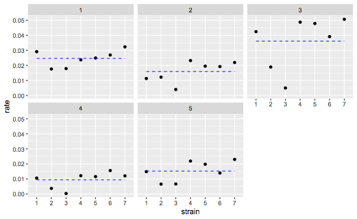
Which should I believe? We can look at the effect of strain and variety:

library(ggplot2)
ggplot(df,aes(x=strain,y=rate)) + geom_point() + geom_smooth(aes(x=as.numeric(strain)),method="lm",
formula=y~1,col="blue",linetype="dashed",se=FALSE,size=0.5)+
facet_wrap(~variety)

From the above, you can see different panels reflect the different variety, the dotted line is the mean of each variety. We can see the strain effect, for example 3 is always lower than the rest, and this is more obvious when we compare across the same variety. Hence we want to put this type of reasoning into practice, by including it into the model.

I hope the above answers "Why do they not agree?". "Which should I believe?" You should use the second model, because if there are variables you know / think can influence the dependent variable, you should include it in, as you can see to properly estimate the between and within group variance.

Answer 2

The 'F' value is the ratio of mean square of strain to that of residual. When the variable, strain alone is there is the model, the ratio for mean square of strain to that of residual is low which means that there is more probability Pr(>F).

When another variable is included in the model, a part (almost 80%) of the residual sum of square in the first model corresponds to the new variable in the model. Thus, the residual sum of square has reduced to a lesser value and so the mean sum of square of the residual. Since, the denominator got reduced, the F value of the variable, strain has become significant.

I tried checking the interaction effect as well. Since the volume of the data is very less where we have only one value for each combinations of strain and variety, I couldn't get the F values and significant values.

If you want to check the interaction effect with different set of data you can do it as below:

mod1<-aov(V7~V2*V1, data=data)
summary(mod1)

For post hoc test

library(lsmeans)
lsmeans(mod1, pairwise ~ V2, adjust="tukey")
lsmeans(mod1, pairwise ~ V1, adjust="tukey")

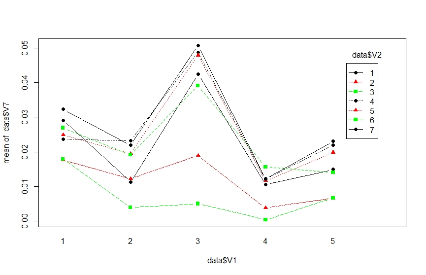
For interaction plot

interaction.plot(x.factor = data$V1, trace.factor = data$V2, response = data$V7, 
                 fun = mean,type="b", col=c("black","red","green"), 
                 pch=c(19, 17, 15),fixed=TRUE, leg.bty = "o")

Interaction Plot