11
$\begingroup$

I'm on a quest for the intuition behind the fact that theoretical introductions to approximate inference focus so much on the log partition function. Say we have a regular exponential family $$p(\mathbf{x};\boldsymbol{\theta}) = \exp\left(\boldsymbol{\phi}(\mathbf{x})^\top\boldsymbol{\theta} - \log Z(\boldsymbol{\theta})\right)$$ with sufficient statistics $\boldsymbol{\phi}(\mathbf{x})$, natural parameters $\boldsymbol{\theta}$, and partition function $Z(\boldsymbol{\theta})$. The partition function is of course defined by $$Z(\boldsymbol{\theta}) = \int\exp\left(\boldsymbol{\phi}(\mathbf{x})^\top\boldsymbol{\theta}\right){\rm d}\mathbf{x} \quad .$$

EDIT: to clarify, the kind of problem I have in mind is where $\mathbf{x}$ is a latent variable in a graphical model with conditional exponential family distributions, as is the focus of Wainwright & Jordan (2008), for instance. Finding an optimal $\boldsymbol{\theta}$ may be a variational inference problem. Conditioned on some data, another common problem would be drawing posterior samples of $\mathbf{x}$.

In my experience, textbooks and tutorials on approximate inference often make claims like "inference is hard because computing the (log) partition function is hard." I don't doubt that computing the log partition function is hard, but I do fail to see why that is "the" barrier to inference.

First, let me explain where I am coming from... To begin, I have a decent grasp of the following:

  1. We need the partition function to compute expected values. If we only know the unnormalized distribution $p^*(\mathbf{x};\boldsymbol{\theta}) = \exp\left(\boldsymbol{\phi}(\mathbf{x})^\top\boldsymbol{\theta}\right)=p(\mathbf{x};\boldsymbol{\theta})Z(\boldsymbol{\theta})$, then we also only know $\mathbb{E}[f(\mathbf{x})]$ up to scaling by $Z(\boldsymbol{\theta})$.
  2. Exact inference is #P-Hard in the worst case.
  3. If we have the gradient of the log partition function, then we have the mapping between natural parameters and mean parameters, $$\nabla_\boldsymbol{\theta} \log Z(\boldsymbol{\theta}) = \mathbb{E}\left[\boldsymbol{\phi}(\mathbf{x})\right]\equiv\boldsymbol{\mu} \quad ,$$ and knowing the mean parameters $\boldsymbol{\mu}$ can aid in other stages of inference or in computing expected values in some circumstances (e.g. if $f$ lies in the span of $\boldsymbol{\phi}$, then $\mathbb{E}[f(\mathbf{x})]$ is linear in $\boldsymbol{\mu}$).

All that being said, I still don't get why computing $\log Z$ is "the" hard problem in inference.

Consider this thought experiment: imagine you are given an oracle who computes $Z(\boldsymbol{\theta})$ efficiently. What can you now do that you could not do before? Take bullet (1) above - can you now compute expected values more easily? It seems to me that there remains a difficult problem, namely computing a high-dimensional integral over $\mathbf{x}$. In fact, much of the space may have negligible probability mass. Personally, I would rather have an oracle that tells me which regions of $\mathbf{x}-$space to look in -- solve the search problem for me, e.g. by providing a set of samples of $\mathbf{x}$ from the posterior or something close to it. Digging into this notion of ``search'' a little deeper, note that this is how Self-Normalized Importance Sampling (SNIS) works: you draw samples from a proposal distribution that is essentially guess about where $\mathbf{x}$ has non-negligible mass, then plug in an estimate of $Z(\boldsymbol{\theta})$ based on those samples, namely $$\hat{Z}(\boldsymbol{\theta}) = \frac{1}{S}\sum_{i=1}^S p^*(\mathbf{x}^{(i)};\boldsymbol{\theta}) \qquad \mathbf{x}^{(i)}\sim q(\mathbf{x})\quad.$$ The hard problem in SNIS is constructing a good proposal distribution $q$, then you get $Z(\boldsymbol{\theta})$ "for free."

One way to find the relevant regions of $\mathbf{x}$ would be to find the mode(s) of $p$. This means solving $$\nabla_\mathbf{x} \log p(\mathbf{x};\boldsymbol{\theta}) = \boldsymbol{\theta}^\top\nabla_\mathbf{x}\boldsymbol{\phi}(\mathbf{x}) = \mathbf{0} $$ (some abuse of notation here... you get the idea). But the difficulty of this depends on $\boldsymbol{\phi}$; the partition function is not involved.

To summarize, I see inference as having two core problems: (a) a search problem for the relevant region of $\mathbf{x}$ (high-probability regions, modes, etc.), and (b) a normalization problem of computing (log) $Z(\boldsymbol{\theta})$. I am puzzled why the latter (b) receives so much attention, especially since solving (a) can give (b) for free, but not the other way around as far as I can tell. So, what is the intuition behind the emphasis on the log partition function?

$\endgroup$
3
  • 1
    $\begingroup$ in your final comment, (a) and (b) are in a sense quite unrelated. at a high level, (a) is about optimisation, and (b) is about integration. roughly speaking, being able to compute partition functions should be useful for integration tasks (computing expectations, marginals, conditional distributions, sampling). see section 1.5 of web.stanford.edu/~montanar/TEACHING/Stat375/handouts/… for details on how these reduce to one another. $\endgroup$
    – πr8
    Commented Jun 5, 2020 at 15:44
  • 1
    $\begingroup$ speculatively: i would guess that computing the partition function is often singled out as "the" hard task because it somehow requires the least extra detail to be explained - you don't need to be looking for a specific { marginal / conditional } distribution, or for the integral of a specific function; it's 'just' a normalising constant, which 'just exists' without extra detail. $\endgroup$
    – πr8
    Commented Jun 5, 2020 at 15:49
  • $\begingroup$ @πr8 the pdf handout looks very relevant, but also very dense. If I had been planning better I wouldn't have put a bounty on this question that expires during a week when I'm extremely busy. But it looks promising and I hope to have a chance to work through it at the proper pace sometime later. A high-level tl;dr as an answer below would be greatly appreciated! $\endgroup$
    – wrongu
    Commented Jun 7, 2020 at 0:59

2 Answers 2

3
+25
$\begingroup$

This is how Self-Normalized Importance Sampling (SNIS) works - you draw samples from a proposal distribution that is essentially guess about where

This shows how the lack of knowledge about $\log Z$ can be solved.

But it doesn't mean that lack of knowledge of $\log Z$ is not a problem.

In fact the SNIS method shows that not knowing $\log Z$ is a problem. It is a problem and we need to use a trick in order to solve it. If we knew $\log Z$ then our sampling method would perform better.

Example

See for instance in the example below where we have a beta distributed variable

$$f_X(x) \propto x^2 \quad \qquad \qquad \text{for $\quad 0 \leq x \leq 1$}$$

And we wish to estimate the expectation value for $log(X)$.

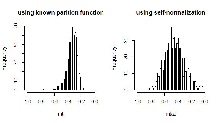
Because this is a simple example we know that $E_X[log(X)] = -1/3$ by calculating it analytically. But here we are gonna use self-normalized importance sampling and sampling with another beta distribution $f_Y(y) \propto (1-y)^2$ to illustrate the difference.

  • In one case we compute it with an exact normalization factor. We can do this because we know $log(Z)$, as for a beta distribution it is not so difficult.

    $$E_X[log(X)] \approx \frac{\sum_{\forall y_i} log(y_i) \frac{y_i^2}{(1-y_i)^2}}{1}$$

  • In the other case we compute it with self-normalization

    $$E_X[log(X)] \approx \frac{\sum_{\forall y_i} log(y_i) \frac{y_i^2}{(1-y_i)^2}}{\sum_{\forall y_i} \frac{y_i^2}{(1-y_i)^2}}$$

So the difference is whether this factor in the denominator is a constant based on the partition function $\log(Z)$ (or actually ratio of partition functions for X and Y), or a random variable $\sum_{\forall y_i} {y_i^2}/{(1-y_i)^2}$.

Intuitively you may guess that this latter will increase bias and variance of the estimate.

The image below gives the histograms for estimates with samples of size 100.

comparison of self-normalization or direct computation of Z

ns <- 100
nt <- 10^3

mt <- rep(0,nt)
zt <- rep(0,nt)

for (i in 1:nt) {
  y <- rbeta(ns,1,3)
  t <- log(y)*y^2/(1-y)^2
  z <- y^2/(1-y)^2
  mt[i] <- mean(t)
  zt[i] <- mean(z)
}

h1 <- hist(mt, breaks = seq(-1,0,0.01), main = "using known parition function")
h2 <- hist(mt/zt , breaks = seq(-1,0,0.01), main = "using self-normalization")
$\endgroup$
6
  • $\begingroup$ Many thanks for the answer and simulations! This is a great example of how knowing Z is better than not knowing it. But I have two outstanding issues. First, I think the more fair comparison here in the spirit of the original question would be to set the proposal distribution to the true beta (solve the "search" problem but leave Z unknown). Second and more important, showing that Z is useful hasn't convinced me that it's more fundamental than solving the "search" problem. Given the choice between a "proposal distribution oracle" and a "Z" oracle, I'd take the proposal oracle -- would you? $\endgroup$
    – wrongu
    Commented Jun 7, 2020 at 0:56
  • $\begingroup$ @wrongu I am not so sure about the question what is more important. I would guess that there is not anything more important or difficult than another thing. But I have not so much experience with textbooks and tutorials to know about the claims that you are referring to (maybe you could give a specific example). So my answer is not really about that, and I was only giving a partial answer that focussed on your example. I am not so sure what you are trying to say with that example since SNIS is very explicitly a way to actually compute $Z$ and in that way confirmation that it is important... $\endgroup$ Commented Jun 7, 2020 at 9:27
  • $\begingroup$ ... in SNIS you compute $Z$ by sampling. My answer shows that this introduces more variation in the estimate/result in comparison to a direct analytical solution. The same would be true for more realistic examples. Whether this makes 'knowing Z' the most important or most difficult problem I do not know. But it is a problem. $\endgroup$ Commented Jun 7, 2020 at 9:49
  • $\begingroup$ My SNIS example was intended to point out what seems to be an asymmetry between two problems: a set of samples of x are sufficient to get a "good enough" estimate of Z, but knowing Z is not enough to say where good samples of x might be. I'm not so much claiming these things as facts as I am trying to communicate an intuition, and wondering where my intuition has gone wrong (if at all). Sorry if this did not come across well in the initial question. $\endgroup$
    – wrongu
    Commented Jun 7, 2020 at 15:13
  • $\begingroup$ I have difficulties imagining a situation where you do not know the relative probability as a function of $x$. This is indeed a prerequisite and indeed the 'not knowing Z' can be "solved" computationally by sampling, but not knowing the distribution is a very difficult problem (actually, I can imagine cases where we do not know exactly the distribution e.g. compound distributions). $\endgroup$ Commented Jun 7, 2020 at 16:20
0
$\begingroup$

As a precursor: It is worth thinking about how these problems arise in statistical practice. Optimising over $x$ is rare - usually, $x$ has already been observed. It is more common to be optimising over $\boldsymbol{\theta}$, given an observation $x$, e.g. to find the maximum likelihood estimator of $\theta$, one would solve

$$\max_\boldsymbol{\theta} \left\{ \log p(\mathbf{x};\boldsymbol{\theta}) = \boldsymbol{\phi}(\mathbf{x})^\top\boldsymbol{\theta} - \log Z(\boldsymbol{\theta}) \right\}.$$

If one is aiming to optimise this function, it is clear that one needs some sort of control on $Z(\boldsymbol{\theta})$, and/or its derivatives.

To address your specific comments:

Consider this thought experiment: imagine you are given an oracle who computes $Z(\boldsymbol{\theta})$ efficiently. What can you now do that you could not do before? [...] can you now compute expected values more easily?

Indeed you can. If you have oracle access to $Z(\boldsymbol{\theta})$, then you can also estimate its gradient by finite differencing. This lets you compute the specific expectation

$$\nabla_\boldsymbol{\theta} \log Z(\boldsymbol{\theta}) = \mathbb{E}\left[\boldsymbol{\phi}(\mathbf{x})\right]\equiv\boldsymbol{\mu}.$$

It does not allow you to compute arbitrary expectations (unless you change to thinking about a different exponential family), but one is typically not looking for arbitrary expectations.

Personally, I would rather have an oracle that tells me which regions of $\mathbf{x}-$space to look in -- solve the search problem for me.

What would this mean? This seems very close to being able to sample from $p(\mathbf{x};\boldsymbol{\theta})$, which is of similar difficulty to computing $Z(\boldsymbol{\theta})$. I agree that this would be a useful oracle, but it is not an easier one.

This is how Self-Normalized Importance Sampling (SNIS) works - you draw samples from a proposal distribution that is essentially guess about where $\mathbf{x}$ has non-negligible mass, then plug in an estimate of $Z(\boldsymbol{\theta})$ based on those samples. The hard problem in SNIS is constructing a good proposal distribution $q$, then you get $Z(\boldsymbol{\theta})$ "for free."

Yes. For many problems of interest, constructing a good $q$ is very difficult, and is usually more difficult than computing $Z(\boldsymbol{\theta})$.

One way to find the relevant regions of $\mathbf{x}$ would be to find the mode(s) of $p$. [...] But the difficulty of this depends on $\boldsymbol{\phi}$; the partition function is not involved.

The extent to which this is useful will depend on the problem at hand. For calculation of expectations, in high-dimensional problems of interest, modes are not as useful as one might think, unless $p$ is very well-concentrated. The difficulty is in integration over the (many) possible states.

To summarize, I see inference as having two core problems: (a) a search problem for the relevant region of $\mathbf{x}$ (high-probability regions, modes, etc.), and (b) a normalization problem of computing (log) $Z(\boldsymbol{\theta})$. I am puzzled why the latter (b) receives so much attention, especially since solving (a) can give (b) for free, but not the other way around as far as I can tell. So, what is the intuition behind the emphasis on the log partition function?

To recapitulate: (a) does not give (b) for free, nor does (b) give (a) for free.

  • (a) is a problem of optimisation over $x$, which does not depend (as much) on the value of $\boldsymbol{\theta}$.
  • (b) is a problem of integration over $x$, which depends intimately on the value of $\boldsymbol{\theta}$.

As stated at the top of this post: statistically, you are usually interested in inference over $\theta$, and $x$ is given already. It is thus more common to be in a situation where (b) is relevant.

$\endgroup$
3
  • $\begingroup$ Thanks for the answer! I now realize was making some unstated assumptions... The kind of statistical practice I have in mind is one where x is a latent variable in a graphical model rather than observed data. If some data y are observed and p(x) is conjugate to the likelihood p(y|x), then what I'm calling the "search" problem over x is finding regions of high posterior probability (or finding an optimal θ parameterizes an approximate variational posterior). Of interest, then, are expected values of arbitrary functions of x. Does this clarify (a) and (b)? $\endgroup$
    – wrongu
    Commented Jun 7, 2020 at 15:22
  • $\begingroup$ (Main question edited to reflect this...) $\endgroup$
    – wrongu
    Commented Jun 7, 2020 at 15:31
  • 1
    $\begingroup$ @wrongu It would be useful if you could give a more concrete example of the type of problem which you have in mind, where the role of the partition function is unclear. $\endgroup$
    – πr8
    Commented Jun 7, 2020 at 16:49

Your Answer

By clicking “Post Your Answer”, you agree to our terms of service and acknowledge you have read our privacy policy.

Not the answer you're looking for? Browse other questions tagged or ask your own question.