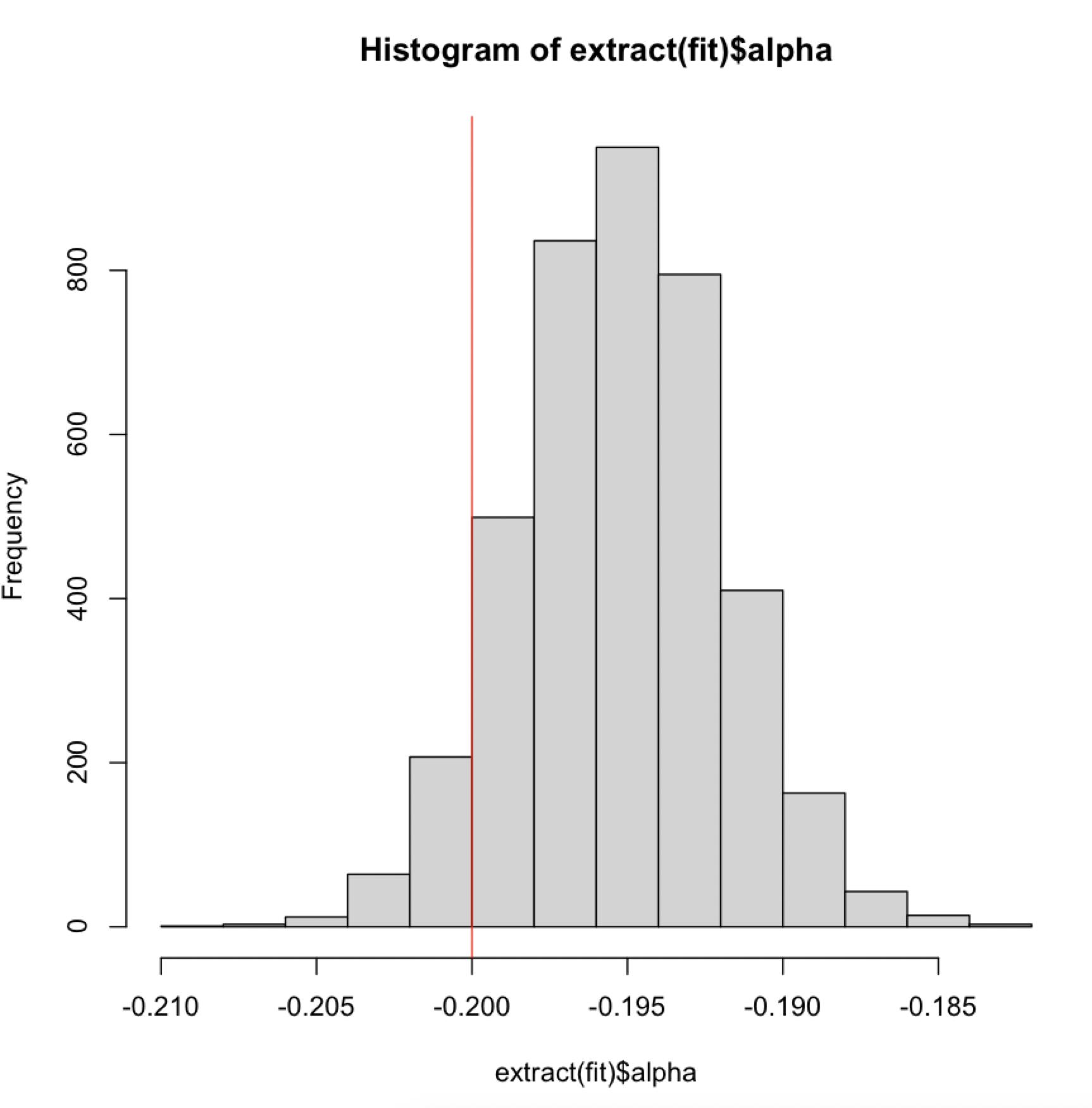
[Note on cross-posting: This question has now been posted on the Stan Forums as well.]
I want to model the index called Delta P (e.g., p.144 of this paper), which is basically a difference between two proportions (i.e., $\frac{n_1}{N_1}$ - $\frac{n_2}{N_2}$), as a function of a predictor. The input data should be the four count variables from which to calculate Delta P (i.e., $n_1$, $N_1$, $n_2$, $N_2$) and predictor values.
Below is my attempt to do it in Stan. When I run the code, I get a message about Jacobian adjustments since the left-hand side of a sampling statement is deltaP, which is calculated by subtracting one parameter from another (theta1 - theta2, where theta1 is the estimated value of $\frac{n_1}{N_1}$ and theta2 is that of $\frac{n_2}{N_2}$).
data {
  int<lower=0> N; // total number of observations
  int<lower=1> denom1[N]; // denominator of the first proportion
  int<lower=1> denom2[N]; // denominator of the second proportion
  int<lower=0> nom1[N]; // nominator of the first proportion
  int<lower=0> nom2[N]; // nominator of the second proportion
  real x[N]; // predictor variable
}

parameters {
  real<lower=0, upper=1> theta1[N]; // the first proportion
  real<lower=0, upper=1> theta2[N]; // the second proportion
  real alpha; // intercept
  real beta; // slope parameter for x
  real<lower=0> sigma; // SD of the error term
}

transformed parameters {
  real<lower=-1, upper=1> deltaP[N]; // Delta P
  for (i in 1:N) {
    deltaP[i] = theta1[i] - theta2[i];
  }
}

model {
  // priors
  theta1 ~ beta(1, 1);
  theta2 ~ beta(1, 1);
  alpha ~ normal(0, 2);
  beta ~ normal(0, 2);
  sigma ~ normal(0, 1) T[0, ];

  for (i in 1:N) {
    // estimating thetas based on denoms and noms
    nom1[i] ~ binomial(denom1[i], theta1[i]);
    nom2[i] ~ binomial(denom2[i], theta2[i]);
    // deltaP is sampled from the truncated normal distribution whose mean is alpha + beta * x and the SD is sigma
    deltaP[i] ~ normal(alpha + beta * x[i], sigma) T[-1, 1];
  }
}
I run the Stan code above with the following R code.
library("rstan")

### Generate fake data
set.seed(100)
# sample size
N <- 100
# True parameter values
alpha <- -0.2
beta <- 0.5
sigma <- 0.1

# predictor values (x) and Delta P values
while (TRUE) {
  x <- runif(N, -1, 1)
  deltaP <- alpha + beta * x + rnorm(N, sd = sigma)
  if (all(deltaP <= 1) & all(deltaP >= -1)) break
}
# theta values
theta1 <- theta2 <- numeric(N)
for (i in 1:N) {
  if (deltaP[i] > 0) {
    theta1[i] <- runif(1, deltaP[i], 1)
    theta2[i] <- theta1[i] - deltaP[i]
  } else {
    theta2[i] <- runif(1, abs(deltaP[i]), 1)
    theta1[i] <- theta2[i] + deltaP[i]
  }
}

# denoms and noms
denom1 <- sample(N, replace = TRUE)
denom2 <- sample(N, replace = TRUE)
nom1 <- rbinom(N, denom1, theta1)
nom2 <- rbinom(N, denom2, theta2)

### fit the model
fit <- stan(file = 'xxx.stan',
            data = list(
              N = N,
              denom1 = denom1,
              denom2 = denom2,
              nom1 = nom1,
              nom2 = nom2,
              x = x
            ))
This runs, but I also get the following message:
DIAGNOSTIC(S) FROM PARSER:
Info:
Left-hand side of sampling statement (~) may contain a non-linear transform of a parameter or local variable.
If it does, you need to include a target += statement with the log absolute determinant of the Jacobian of the transform.
Left-hand-side of sampling statement:
    deltaP[i] ~ normal(...)
I only have a vague understanding of Jacobian, but I believe it is necessary when parameters are transformed nonlinearly as it alters the shape of variable distribution. What I am not sure of is whether the case above (deltaP = theta1 - theta2) equates with nonlinear transformation, and if it does, what kind of Jacobian adjustments are necessary (or if there are any other ways to circumvent the issue).
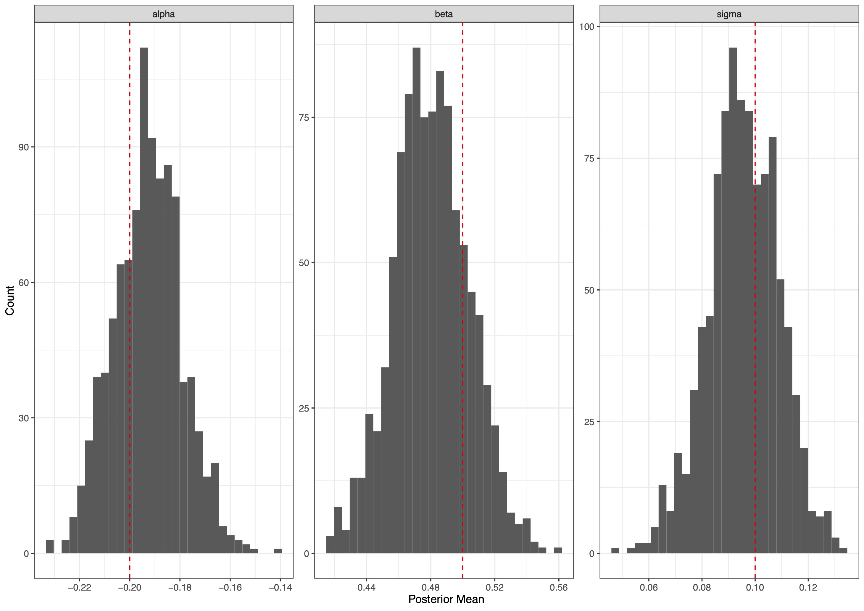
When I repeated the above code 1,000 times with different seeds and examined the distribution of the mean of the posterior distributions in the three focal parameters (i.e., alpha, beta, sigma), 70.5% of alpha, 20.1% of beta, and 37.4% of sigma were above the true value (see figure below), which makes me suspect they may be biased and the bias could be due to the lack of Jacobian adjustments.


