Autocorrelation in linear mixed models (lme)

Question

To study the diving behaviour of whales, I have a dataframe where each row corresponds to a dive (id) carried out by a tagged individual (whale). For each dive I calculate a series of parameters (maximum depth, duration, etc.).

# Example dataframe
id whale max_depths duration pd_times    d_rate     a_rate    bottom_dur  bottom_prop dive_type  diel   
1   1         57      166       41      0.5288462  0.9152542          2     1.2048193         F  Day
2   1         26      165       43      0.2688172  0.3333333          2     1.2121212        NF  Day
3   1         18      140       90      0.1911765  0.3500000         31    22.1428571        NF  Day

There are two type of dives ( F in which the whale feeds and NF where there is no feeding activity)

I want to compare all parameters between F and NF dives.

For that, I started by trying to apply a linear mixed model for each parameter with whale number as random effect and diel (since their behaviour may change according to time of day) as fixed effect (code below):

Diel -> in this column it is specified at what time of day the dive was carried out (for example, in one day if the sunrise is at 6:00h and sunset at 20:00h:

• from 6:00 - 19:00h = "Day"
• from 19:00 - 20:00h = "Twilight" (in this case "Dusk")
• from 20:00h till the begin of "Dawn" of the next day is "Night" and this continues based on local sunrise/sunset values

So if a dive was carried out at 18:00h of that day, in diel it would be "Day" and if the next dive was carried out at 19:15h it would be in the "Night" category.

    model_3 <- lme(duration ~ dive_type + diel_1, random=~1 | whale,method = "REML",
                   data = data,na.action=na.exclude)
    summary(model_3)
    AIC(model_3) 
    plot(model_3) 

> summary(model_1)
Linear mixed-effects model fit by REML
 Data: data 
       AIC      BIC    logLik
  33143.93 33167.49 -16567.96

Random effects:
 Formula: ~1 | whale
        (Intercept) Residual
StdDev:    92.03755 116.9184

Fixed effects: duration ~ dive_type 
                Value Std.Error   DF   t-value p-value
(Intercept) 291.57762 20.491341 2653  14.22931       0
dive_typeNF -61.55134  4.656191 2653 -13.21925       0
 Correlation: 
            (Intr)
dive_typeNF -0.123

Standardized Within-Group Residuals:
       Min         Q1        Med         Q3        Max 
-3.2584814 -0.7034402 -0.1069537  0.5686564  5.4987687 

Number of Observations: 2675
Number of Groups: 21 

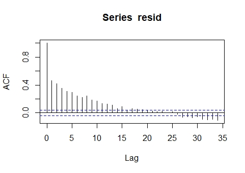
When I plotted the residuals I found they were not normal and there was a high level of autocorrelation (graph below)

After tranforming the data (log) the distribution seems closer to normal but there is still a high autocorrelation.

To try to fix these issue I included the corAR1 function as follow:

model_6_cor_2 <- lme(duration ~ dive_type  + diel_1, random=~1 | whale,method = "REML",
                   data = data,
                   #correlation=corARMA(p=2,q=0),
                   correlation = corAR1(form = ~ 1 | whale),
                   na.action=na.exclude)
summary(model_6_cor_2)
AIC(model_6_cor_2) 

But the autocorrelation plot remains basically the same.

I tried a GLM with Poisson and negative binomial distribution and the problem remains.

What can I do to solve this issue?

Thank you in advance.

Answer 1

Gavin Simpson raised a good point in the comment that there are several types of residuals to plot: regular, standardized, and normalized. You want to use the normalized one to plot if you want to examine how much of autocorrelation is resolved by a first-order auto-regression process, such as plot(ACF(model, maxLag = 78, resType = "normalized"), alpha = 0.05).

Usually either random effects or autocorrelation should be modeled by the same grouping indicator but not both. If you already have a random intercept varying by whale, it already captures the correlation between multiple measurements taken from the same whale, so it will be redundant to use autocorrelation. In fact, you will probably see that either the random-effect standard deviation is zero or the autocorrelation coefficient is at boundaries, if you keep both terms in the model. Use intervals to check if at least one of them cannot be accurately estimated. You can compare whether random effects or autocorrelation is a better choice by using anova() or AIC.

But before you start to worry about autocorrelation, make sure that you sort the observations in the correct order, as lme() by default use the implicit row index as the time indicator. See other modeling procedures in my answer Is it possible to calculate x-intercept from a mixed model?. In your case, dive duration and depth are both positive integers, you can model them as (1) count model, perhaps zero truncated (2) survival analysis, such as Cox proportional hazard model (3) gamma regression (4) ordinal regression. With the predictors, it is possible and perhaps very useful to include season as categorical and year as numeric predictors, then you may discover astonishing findings such as "whales do dive as deep as they used to, possibly due to food scarcity, vessel disturbance, and marine pollution."