Both are estimators that maximize the marginal likelihood, only GLMM does so by first considering the conditional probability, while GEE assumes a covariance structure of the marginal probability directly. So why should the coefficients be systematically different one from the other (GEE gives coefficients that are smaller in magnitude)?
1 Answer
This actually depends on the link function -- eg, for a log link there is not a systematic difference, but for a logit link there is.
The reason is that the models are systematically different and the marginal likelihoods are systematically different. As the simplest example consider a logistic GLMM with a random intercept, for longitudinal data indexed by person $i$ and time $t$
$$\mathrm{logit} E[Y_{it}|X_{it}=x, a_i] = a_i+x\beta$$ where $a_i\sim N(\alpha, \tau^2)$
The GEE marginal mean model is
$$\mathrm{logit} E[Y_{it}|X_{it}]=\tilde\alpha+x\tilde\beta$$
So how are $\beta$ and $\tilde\beta$ related? Well, the GLMM has $$E[Y_{it}|X_{it}=x, a_i] = \mathrm{expit}\,(a_i+x\beta)$$ so $$E[Y_{it}|X_{it}=x] = E_a[E[Y_{it}|X_{it}=x, a_i]]=E_a[\mathrm{expit}\,(a_i+x\beta)]$$ so $$\mathrm{logit}\, E[Y_{it}|X_{it}=x] = \mathrm{logit}\,E_a[\mathrm{expit}\,(a_i+x\beta)]$$
The GEE has $$\mathrm{logit} E[Y_{it}|X_{it}=\tilde\alpha+x\tilde\beta$$
These would be the same if expectations and $\mathrm{expit}$ commuted, but they don't. For a log link, the $\beta$ would be the same, because you can take an $e^\beta$ multiplier through the expectation, but the $\alpha$ would be systematically different.
Ok, so we know $\beta\neq\tilde\beta$ (for the true parameters, not just the estimates). Why is $|\beta|>|\tilde\beta|$?
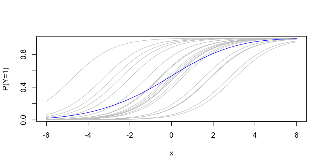
I think this is easiest with a picture
expit<- function(x) exp(x)/(1+exp(x))

x<-seq(-6,6,length=50)
eta_c <- 0+1*x
mu_c <- expit(eta_m)
plot(x, mu_c,ylab="P(Y=1)",lwd=2,type="n",xlim=c(-6,6))

a<-rnorm(20,s=2)

total_m<-numeric(50)
for(ai in a){
  eta_c <- ai+0+1*x
  mu_c <- expit(eta_c)
  lines(x, mu_c, col="grey")
  total_m<-total_m+mu_c
}

mu_m<-total_m/20
lines(x, mu_m, col="blue")
What we see here is 20 realisations in grey of the conditional mean functions for 20 random $a_i$, and the blue curve that is the average of the grey curves, which is the GEE mean curve. They are basically the same shape, but the population-average curve is flatter; $\tilde\beta<\beta$.
The grey curves are all the same shape. The derivative of $p= \mathrm{expit}\eta$ wrt $\eta$ is $$\frac{\partial p}{\partial\eta} = \mathrm{expit}\eta$ (1-\mathrm{expit}\eta)=p(1-p)$$ so $$\frac{\partial p}{\partial x} = p(1-p)\frac{\partial\eta}{\partial x}=p(1-p)\beta$$ That is, the grey curves all have slope $\beta/4$ where they cross $p=0.5$ and the blue curve will have slope $\tilde\beta/4$.
One issue I've avoided here is that the GEE and GLMM logistic models are incompatible; they can't both be exactly true. But you could pretend that I used a probit link instead, where they are compatible, or that I'd looked up the relevant bridge distribution to replace the Normal distribution for $a_i$.
-
$\begingroup$ didn't expect such a thorough reply so quickly :-) $\endgroup$ Commented Sep 6, 2020 at 8:28
-
$\begingroup$ Is the graph comparing the right things, though? It seems to me that you are comparing the conditional GLMM with the marginal GLMM... $\endgroup$ Commented Sep 6, 2020 at 8:32
-
$\begingroup$ The slope of the grey curves where they cross 0.5 is proportional to $\beta$; the slope of the blue curve where it crosses 0.5 is proportional to $\tilde\beta$ (with the same proportionality constant) $\endgroup$ Commented Sep 6, 2020 at 8:44
-
$\begingroup$ Is there some proof of that? $\endgroup$ Commented Sep 6, 2020 at 12:28

