Sum of squares of residuals instead of sum of residuals [duplicate]

Question

As I was working my way through my book about statistics, I came across the topic of linear regression. During the chapter the author begins with explaining that you want to minimize the residuals in order to make your y = a + bx as good a fit as possible: I do understand this, but halfway the chapter all of a sudden the residuals change into sum squares of residuals. Why is this done? I have been googling, but couldn't find the right answer. Who would like to help me understand why the sums of squares of the residuals is used instead of just the sums of residuals?

Kind regards, Bas

Answer 1

The sums of residuals will always be 0, so that won't work.

A more interesting question is why use sum of squared residuals vs. sum of absolute value of residuals. This penalizes large residuals more than small ones. I believe the reason this is done is because the math works out more easily and, back before computers, it was much easier to estimate the regression using squared residuals. Nowadays, this reason no longer applies mean absolute deviation regression is, indeed, possible. It is one form of robust regression.

Answer 2

Another way to motivate the squared residuals is by making the often reasonable assumption that the residuals are Gaussian distributed. In other words, we assume that $$y = ax + b + \varepsilon$$ for Gaussian noise $\varepsilon$. In this case, the log-likelihood of the parameters $a, b$ is given by $$\log p(y \mid x, a, b) = \log \mathcal{N}(y; ax + b, 1) = -\frac{1}{2} (y - [a + bx])^2 + \text{const},$$ so that maximizing the likelihood amounts to minimizing the squared residuals.

If the noise $\varepsilon$ was Laplace distributed, the absolute value of residuals would be more appropriate. But because of the central limit theorem, Gaussian noise is much more common.

Answer 3

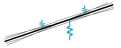
Good answers, but maybe I can give a more intuitive answer. Suppose you are fitting a linear model, represented here by a straight line parameterized by a slope and intercept.

Each residual is a spring between each data point and the line, and it is trying to pull the line to itself.
A sensible thing to do is find the slope and intercept that minimizes the energy of the system. The energy in each spring (i.e. residual) is proportional to its length squared. So what the system does is minimize the sum of the squared residuals, i.e. minimize the sum of energy in the springs.

Answer 4

This is more a response to @PeterFlom's comment on my comment, but it is too big to fit in a comment (and does relate to the original question).

Here is some R code to show a case where there are multiple lines that all give the same minimum MAD/SAD values.

The first part of the example is clearly contrived data to demonstrate, but the end includes more of a random element to demonstrate that the general concept will still hold in some more realistic cases.

x <- rep(1:10, each=2)
y <- x/10 + 0:1
plot(x,y)
    
sad <- function(x,y,coef) { # mad is sad/n
        yhat <- coef[1] + coef[2]*x
        resid <- y - yhat
        sum( abs( resid ) )
    }
    
library(quantreg)
fit0 <- rq( y~x )
abline(fit0)
    
fit1 <- lm( y~x, subset= c(1,20) )
fit2 <- lm( y~x, subset= c(2,19) )
fit3 <- lm( y~x, subset= c(2,20) )
fit4 <- lm( y~x, subset= c(1,19) )
    
fit5.coef <- c(0.5, 1/10)
    
abline(fit1)
abline(fit2)
abline(fit3)
abline(fit4)
abline(fit5.coef)
for (i in seq( -0.5, 0.5, by=0.1 ) ) {
        abline( fit5.coef + c(i,0) )
    }
    
tmp1 <- seq( coef(fit1)[1], coef(fit2)[1], len=10 )
tmp2 <- seq( coef(fit1)[2], coef(fit2)[2], len=10 )
    
for (i in seq_along(tmp1) ) {
        abline( tmp1[i], tmp2[i] )
    }
    
sad(x,y, coef(fit0))
sad(x,y, coef(fit1))
sad(x,y, coef(fit2))
sad(x,y, coef(fit3))
sad(x,y, coef(fit4))
sad(x,y, fit5.coef )
    
for (i in seq( -0.5, 0.5, by=0.1 ) ) {
        print(sad(x,y, fit5.coef + c(i,0) ))
    }
    
for (i in seq_along(tmp1) ) {
        print(sad(x,y, c(tmp1[i], tmp2[i]) ) )
    }
    
set.seed(1)
y2 <- y + rnorm(20,0,0.25)
plot(x,y2)
fitnew <- rq(y2~x)  # note the still non-unique warning
abline(fitnew)
abline(coef(fitnew) + c(.1,0))
abline(coef(fitnew) + c(0, 0.01) )
sad( x,y2, coef(fitnew) )
sad( x,y2, coef(fitnew)+c(.1,0))
sad( x,y2, coef(fitnew)+c(0,0.01))

Answer 5

In addition to the points made by Peter Flom and Lucas, a reason for minimizing the sum of squared residuals is the Gauss-Markov Theorem. This says that if the assumptions of classical linear regression are met, then the ordinary least squares estimator is more efficient than any other linear unbiased estimator. 'More efficient' implies that the variances of the estimated coefficients are lower; in other words, the estimated coefficients are more precise. The theorem holds even if the residuals do not have a normal or Gaussian distribution.

However, the theorem is not relevant to the specific comparison between minimizing the sum of absolute values and minimizing the sum of squares since the former is not a linear estimator. See this table contrasting their properties, showing advantages of least squares as stability in response to small changes in data, and always having a single solution.