random effect variance increases with the inclusion of predictor

Question

What does it mean when the inclusion of a fixed effect (sex) increases variance of the random effect?

dat <- data.frame(ID=rep(1:12), sex=c(0,1,1,1,0,0,1,0,1,1,0,1), region=rep(c("A","B"),each=6), y=c(12,13,15,7,8,4,8,8,9,3,4,5))

m <- lmer(y~1+(1|region),data=dat)
VarCorr(m)
 Groups   Name        Std.Dev.
 region   (Intercept) 2.1820    

m = lmer(y~sex+(1|region),data=dat)
VarCorr(m)
 Groups   Name        Std.Dev.
 region   (Intercept) 2.4544 

I thought including an independent variable could only decrease random effect variance, but I am obviously wrong. Is it a good idea to include sex in the model even though it increases random effect variance?

Answer 1

In this case, the expected behaviour is that the variance of the random intercepts will be unchanged after adding the predictor. In reality, it will change, but the expected change is still zero. If we modify your simulation slightly, we can see that it can decrease slightly:

> dat$region <- rep(c("A","B","C"),each=4)

> lmer(y~1+(1|region),data=dat) %>% VarCorr()
## Groups   Name        Std.Dev.
## region   (Intercept) 3.0721  
## Residual             2.7386  

> lmer(y~sex+(1|region),data=dat) %>% VarCorr()
## Groups   Name        Std.Dev.
## region   (Intercept) 3.0236  
## Residual             2.8577 

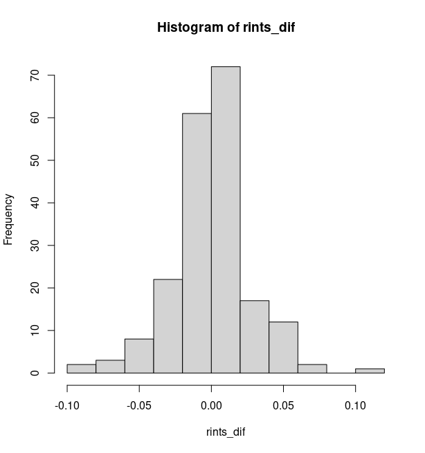
If we were to repeat this, with different data, we would find that, on average the difference will be zero. We can do a simple simulation to show this:

> N <- 100
> n.sim <- 200
> rints_dif <- as.numeric(n.sim)
> for(i in 1:n.sim) {
+   set.seed(i)
+ 
+   X <- rnorm(N) 
+   G <- rbinom(N, 10, 0.5)
+   Y <- G + rnorm(N)
+ 
+   m0 <- lmer(Y ~ 1 + (1|G))
+ 
+   m1 <- lmer(Y ~ 1 + X + (1|G))
+ 
+   rints_dif[i] <- as.data.frame(VarCorr(m0))$sdcor[1] - as.data.frame(VarCorr(m1))$sdcor[1]
+ }
> hist(rints_dif)
> mean(rints_dif)
[1] -0.0002529647

Answer 2

As a quick update to the excellent answer by @RobertLong, I simulated some data in Stata to demonstrate how a predictor that itself has sizable between-cluster variance increases the between-cluster variance in the outcome.

Here are the TLDR results. I simulated x1 so that it has almost no between-school variability whereas x2 was simulated to have a fair bit of it. Notice how in column 2 the sd(school) remains almost the same as in column 1. Contrastingly, in columns 3 and 4, the sd(school) increases substantially relative to column1.

----------------------------------------------------------------
                      (1)          (2)          (3)          (4)
                        y            y            y            y
----------------------------------------------------------------
x2                               1.592                     0.976
                              (0.0685)                  (0.0740)

x1                                            2.342        1.480
                                           (0.0904)      (0.100)

_cons               15.44        11.14        7.478        7.769
                  (0.167)      (0.237)      (0.537)      (0.414)
----------------------------------------------------------------
sd(school)          0.763        0.758        3.034        2.045
                  (0.185)      (0.146)      (0.338)      (0.260)
----------------------------------------------------------------
sd(residual)        4.041        3.242        3.054        2.876
                 (0.0927)     (0.0744)     (0.0703)     (0.0666)
----------------------------------------------------------------
N                    1000         1000         1000         1000
----------------------------------------------------------------
Standard errors in parentheses

Simulation code is below:

version 16.1 
clear *
set seed 683728

* create scalar to be multplied by rnormal() when creating random intercept
scalar sd_sch_id = .5 // ICC = .5/4+.5 = .11
*scalar sd_residual = 4 

* Schools
set obs 50
gen schid = _n 
gen re_sch_id = sd_sch_id*rnormal() // random intercept, school level 

* Students
expand 20 
by schid, sort: gen stuid = _n

* create a vector that contains the equivalent of a lower triangular correlation matrix for x1, x2, and y
matrix c = (1, 0.5968, 1, 0.6623, 0.6174, 1)
* create a vector that contains the means of the variables
matrix m = (3.23,2.775,15.645)
* create a vector that contains the standard deviations
matrix sd = (1.05,1.47,4) 
* draw a sample of 1000 cases from a normal distribution with specified correlation structure and specified means and standard deviations
drawnorm x1 x2 y, n(1000) corr(c) cstorage(lower) means(m) sds(sd)
corr y x1 x2 // looks good

*gen residual = sd_res*rnormal() // not needed b/c resiudal baked into drawnorm 

* Add random effects to x1, x2, and y
egen pick1sch = tag(schid)
*x1 and x2
scalar sd_x1_sch = 1.2
scalar sd_x2_sch = .01
foreach v of varlist x1 x2 {
    gen re_`v'_sch = sd_`v'_sch*rnormal() if pick1sch==1
    bysort schid: replace re_`v'_sch = re_`v'_sch[_n-1] if missing(re_`v'_sch)
    replace `v' = `v' + re_`v'_sch 
}

*y
replace y = y + re_sch_id 

foreach v of varlist x1 x2 y {
    bysort schid: egen sch_mn_`v' = mean(`v')
    gen cws_`v' = `v' - sch_mn_`v'
}

mixed y || schid: , stddev // sd = 0.76
eststo empty
mixed y x2 || schid:, stddev // sd = 0.76
eststo x2
mixed y x1 || schid:, stddev // sd = 3.30
eststo x1
mixed y x1 sch_mn_x1 || schid:, stddev // sd = 0.96

mixed y x1 x2 || schid:, stddev // sd = 2.04
eststo x1_x2