Numbers of draws on a modified Bernouilli process

Question

Here is the setup:

Bob runs an experiment: he flips a coin N times (between 0 and +$\infty$). The coin has a probability p of landing on heads. Bob starts with zero points. For each head, Bob scores a point.

Now, Bob goes to Alice and tells her p and that the score is zero, and ask her the probability that he flipped the coin N=n times.

The case that make it special for me is the addition of the possibility of zero draws, and I'm stuck with it. Here is my attempt at solving this:

N is the random variable counting the number of flips, S is the random variable counting the score.

We want to know $P(N=n|S=0)$.

$$ P(N=n|S=0) = \frac{P(S=0|N=n) \cdot P(N=n)}{P(S=0)} $$

Now $P(S=0|N=n)= (1-p)^{n}$ so that's good.
Also, $P(S=0) = P(N=0) + \sum\limits_{n=1}^\infty (1-p)^{n}P(N=n) $

But now I'm stuck since I don't know what do with that $P(N=n)$. Now you could argue that since we know nothing about the distribution of N, the most reasonable assumption is that they are all equally likely.

Then the substitution occurs as: $$ P(N=n|S=0) = \frac{P(S=0|N=n) \cdot P(N)}{\frac{1}{p}\cdot P(N)} = p(1-p)^{n} $$

This feels like cheating. Not because of the limit, this looks legit cf replace $\infty$ with $N_{max}$ and take the limit at the end, but because of the assumption on $P(N)$ being uniform. While keeping $N_{max}$ this is good, but it seems shady when taking the limit. Also, what do I know if it is uniform ?

Am I doing something wrong here ?

Answer 1

Your algebra seems right, but you are using a noninformative prior distribution, and a very special one at that! A uniform prior on the nonnegative integers gives almost all the mass to extremely large values, which might not be consistent with the fact that Bob have actually been tossing the coin that many times, and do not have unlimited time ... So at least you should do some experiments with alternative priors. First let us try a harmonic prior

$$ \DeclareMathOperator{\P}{\mathbb{P}} \P(N=n)=\frac1{n+1} \qquad, n=0,1,2, \dotsc $$ Unfortunately, that prior is improper, as the sum of the harmonic numbers diverges. So let us truncate it at a maximum value $\bar{N}$. Then we first need

$$ \sum_{n=0}^\bar{N} \frac1{n+1} = H(\bar{N} + 1) = \Psi(\bar{N}+2)+\gamma $$

where $H$ is the harmonic numbers, $\Psi$ the digamma function and $\gamma$ the Euler constant. (I use Maple for help with the calculations here, it becomes quite ugly and even involves a function I just learned now. I do not give then all the details ...) Using this truncated prior, let us calculate

\begin{multline} \P(S=0)=\sum_n (1-p)^n\cdot \P(N=n) = \\ \frac{-\frac{\left(1-p \right)^{N +1} \Phi \left(1-p , 1, N\right)}{\left(1-p \right)^{2}} -\frac{\ln \left(p \right)}{1-p} - \left(1-p \right)^{N +1} \left(-\frac{1}{\left(1-p \right)^{2} N}-\frac{1}{\left(1-p \right) \left(N +1\right)}\right)}{\Psi \! \left(N +2\right)+\gamma} \end{multline} where $\Phi$ is the Lerch transcendent, but that will happily disappear later when we take the limit $\bar{N} \to \infty$. (Here I tried first the shortcut of just using the improper prior as it were proper, but that lead to a posterior not summing to 1). Using this we calculate the posterior:

\begin{multline} \P(N=n\mid S=0)=\frac{\P(S=0\mid N=n)\P(N=n)}{\P(S=0)}= \\ \frac{\left(1-p \right)^{k}}{\left(k +1\right) \left(-\left(1-p \right)^{N -1} \Phi \! \left(1-p , 1, N\right)+\frac{\ln \left(p \right)}{-1+p}-\frac{\left(1-p \right)^{N -1} \left(N p -2 N -1\right)}{N \left(N +1\right)}\right)} \end{multline}
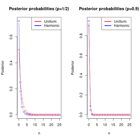
and now taking the limit as $\bar{N}\to\infty$ gives the posterior $$ \P(N=n\mid S=0)=\frac{(1-p)^{n+1}}{(n+1)\log(1/p)} $$ which we now can compare to your posterior $p(1-p)^n$:

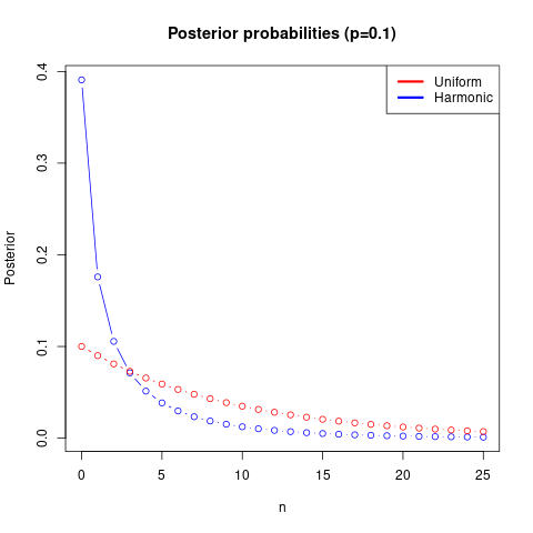
which we have drawn for two values of $p$. Let us finally compare the posteriors for $p=0.1$, a value that makes the observed data $S=0$ more probable than in the first plot. Then the difference between the priors show up:

The uniform prior leads to still maintaining that quite high values of $N$ are possible, while the harmonic prior adapts to data information much faster. For completeness the r code for the last plot:

range <- 0:25

plot(range, harpost(range, 0.1), col="blue", 
     log="", type="b",
     main="Posterior probabilities (p=0.1)", 
     xlab="n", ylab="Posterior")
lines(range, unipost(range, 0.1), col="red", 
      type="b") 

legend("topright", legend=c("Uniform", 
       "Harmonic"), col=c("red", "blue"),
       lwd=3)