Why does my simulation of nearest neighbors as circle origins provide different non-contact probability compared to theoretical?

Question

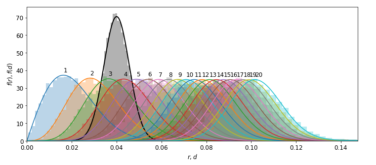
I am simulating spatially distributed points in $\mathbb{R}^2$ with intensity $\lambda$ (units 1/area), which act as circle origins with radii being a random variable $R_k$. Given the distance to the $k$th nearest neighbor $D_k$ (see e.g. Moltchanov 2012), the contact probability of the circle located in the origin (denoted with subscript 0) with the circle originated as the $k$th neighbor is \begin{equation} P(\mathrm{contact \ with \ circle\ } k) = P(R_0 + R_k \ge D_k). \end{equation} As a MWE, I will use $R_k \sim \mathcal{N}(\mu, \sigma^2)$ and Poisson process for spatial. The distance distribution then follows a generalized Gamma distribution \begin{equation} f_{D_k}(r) = \frac{2(\lambda \pi r^2)^k}{r \Gamma(k)}e^{-\lambda \pi r^2}, \quad r > 0, \ k=1,2,\dots \end{equation} The sum distribution of two identical normally distributed radii is \begin{equation} R_0 + R_k \equiv Z \sim \mathcal{N}(2 \mu, 2 \sigma^2) \end{equation} The contact probability is then calculated from \begin{equation} P(\mathrm{contact \ with \ circle\ } k) = \int_{0^+}^\infty f_Z(r) F_{D_k}(r) dr \end{equation} The probability of the circle in the origin not being in contact with any of the $M$ nearest neighbors is then \begin{equation} P(\mathrm{not \ in \ contact \ with \ any}) = \prod_{k=1}^{M}(1-P(\mathrm{contact \ with \ circle\ } k)) \end{equation} The probability of non-contact I get differs from the simulation by quite a big margin (up to >20 times difference), and I fail to understand why?

List of checks performed

• The distance distributions agree with the simulated
• The distribution of the sum of two radii is correct
• In the simulation, I try to eliminate the boundary effects by only considering the circles with origins within some distance from the simulation borders
• Simulation is performed with relatively high $\lambda$, large $A$ and multiple repeats to ensure the variability is not the root cause for the difference

MWE python code and sample outputs

from matplotlib import pyplot as plt
from scipy.stats import poisson, norm, gengamma
from scipy.integrate import trapz
%matplotlib inline

plt.rcParams["font.size"] = 12
np.random.seed(1)
# Circle size parameters
mu = 0.02
sigma = 0.2*mu
# Circle density [1/area]
la = 600.0
A = 20.0 # Area
w = np.sqrt(A) # Width
##############
# Simulation #
##############
N = poisson.rvs(la*A) # Number of circles
xs = np.random.rand(N)*w # Simulated x-coordinates
ys = np.random.rand(N)*w # Simulated y-coordinates
# Border effect - consider only circles that are some distance away from the simulation border
val_ind = (xs >= 0.1*w) & (xs <= 0.9*w) & (ys >= 0.1*w) & (ys <= 0.9*w)
print("N = %i, N_val = %i"%(N, sum(val_ind)))
rs = np.random.randn(N)*sigma + mu # Simulated radii

Ds = np.zeros((N,N)) # Distance matrix
contact = np.zeros((N,N), dtype=bool) # Contact-indicator matrix
for i in range(N):
    Ds[i,:] = np.sqrt((xs[i] - xs)**2 + (ys[i] - ys)**2) # Distances to other circle centers
    contact[i,rs[i] + rs >= Ds[i,:]] = True # Determine which circles are in contact

np.fill_diagonal(contact, False) # Remove self-contact
Ds_sorted = np.sort(Ds) # Sort by distance
contact_counts = np.sum(contact, axis=0)
print("P(no contact) = %.2f%%"%(float(sum(contact_counts[val_ind]==0))/sum(val_ind)*100))

########################
# Prediction and plots #
########################
fig, ax = plt.subplots(figsize=(12.,5.))
rv_z = norm(2.0*mu, np.sqrt(2.0)*sigma) # Sum of two normally distributed radii, both with parameters (mu, sigma)
# Number of nearest neighbors to be considered
M_candidates = np.arange(1,101)
M = M_candidates[np.where(gengamma.ppf(1e-4, M_candidates, 2, scale=(la*np.pi)**(-1.0/2.0)) > rv_z.ppf(1.0 - 1e-4))[0][0]]
r = np.linspace(0.0, gengamma.ppf(1.0-1e-4, M, 2, scale=(la*np.pi)**(-1.0/2.0)), 400) # Distance / radius
# Z = R_i + R_j

fz = rv_z.pdf(r)
Fz = rv_z.cdf(r)
line, = plt.plot(r, fz, 'k-', linewidth=2)
rs2 = rs.copy()
np.random.shuffle(rs2)
zs = rs + rs2 # Simulate sum of two radii
plt.hist(zs, bins=50, density=True, color=line.get_color(), alpha=0.3)

ps = np.zeros(M) # Probabilities of being in contact with ith nearest circle
for i in range(1, M+1):
    fd = gengamma.pdf(r, i, 2, scale=(la*np.pi)**(-1.0/2.0)) # Distance to ith neighbour pdf
    Fd = gengamma.cdf(r, i, 2, scale=(la*np.pi)**(-1.0/2.0)) # Distance to ith neighbour cdf
    line, = plt.plot(r, fd)
    plt.text(r[np.argmax(fd)], 1.05*np.max(fd), str(i))
    plt.hist(Ds_sorted[:,i], bins=50, density=True, alpha=0.3, color=line.get_color()) # Simulated distances to ith
    ps[i-1] = trapz(Fd*fz, r) # P(contact) = P(R_0 + R_i \ge D_i)
    print("i = %i, P(contact with circle %i) = %f%%"%(i, i, ps[i-1]*100))

plt.xlim([0.0, r.max()])
plt.xlabel("$r,d$")
plt.ylabel("$f(r), f(d)$")
print("P(no contact to any of the circles) = %.2f%%"%((np.prod(1.0-ps))*100))

with output prints

N = 11974, N_val = 7715
P(no contact) = 6.21%
i = 1, P(contact with circle 1) = 93.595769%
i = 2, P(contact with circle 2) = 77.871000%
i = 3, P(contact with circle 3) = 56.891694%
i = 4, P(contact with circle 4) = 36.800897%
i = 5, P(contact with circle 5) = 21.376076%
i = 6, P(contact with circle 6) = 11.307534%
i = 7, P(contact with circle 7) = 5.514789%
i = 8, P(contact with circle 8) = 2.505546%
i = 9, P(contact with circle 9) = 1.069581%
i = 10, P(contact with circle 10) = 0.432070%
i = 11, P(contact with circle 11) = 0.166151%
i = 12, P(contact with circle 12) = 0.061127%
i = 13, P(contact with circle 13) = 0.021606%
i = 14, P(contact with circle 14) = 0.007364%
i = 15, P(contact with circle 15) = 0.002428%
i = 16, P(contact with circle 16) = 0.000776%
i = 17, P(contact with circle 17) = 0.000241%
i = 18, P(contact with circle 18) = 0.000073%
i = 19, P(contact with circle 19) = 0.000022%
i = 20, P(contact with circle 20) = 0.000006%
P(no contact to any of the circles) = 0.24%

And output plot with the distribution of two radii added together as black thicker line and the distances to $k$th neighbor, both predicted (continuous lines) and simulated (histograms):

So the predicted non-contact probability is 0.24% whereas the simulated is 6.21%. So there is obviously something wrong with my analysis/simulation. The distributions shown in the plot above indicate that the predicted non-contact probability is plausible.

Answer 1

Given a circular inspection area described by a radius $R$ filled with points from Poisson process, the cumulative density function for distances to the origin is \begin{equation} F_{ro}(r) = \frac{r^2}{R^2} \end{equation} The number of points follows Poisson distribution $N \sim \mathrm{Poi}(\lambda \pi R^2)$ points that act as circle origins with radius pdf $f_r(r)$, we calculate the probability that all $N$ points are further away from the origin than $r_0 + r_j$: \begin{equation} \int \int \dots \int \left(1 - \left(\frac{r_0 + r_1}{R}\right)^2 \right) f_{r}(r_1) \left(1 - \left(\frac{r_0 + r_2}{R}\right)^2 \right) f_{r}(r_2)\dots \left(1 - \left(\frac{r_0 + r_n}{R}\right)^2 \right) f_{r}(r_n) f_r(r_0) dr_0dr_1dr_2 \dots dr_n \end{equation} In the integrand, we see the term repeating \begin{equation} g(r_0) = \int_0^{R - r_0} \left(1 - \left(\frac{r_0 + r_j}{R}\right)^2 \right) f_{r}(r_j) dr_j \end{equation} Expanding the terms, we get \begin{equation} g(r_0) = \int_0^{R-r_0} \left(1 - \frac{r_0^2}{R^2} \right) f_{r}(r_j) dr_j - \int_0^{R-r_0} \frac{2r_0 r_j}{R^2} f_{r}(r_j) dr_j - \int_0^{R-r_0} \frac{r_j^2}{R^2} f_{r}(r_j) dr_j \end{equation} Assuming $R \gg r_j$ so the whole support of $f_r$ is covered by the integrals, we can use the moments. For Normally distributed radius, used in the MWE: \begin{equation} g(r_0) = 1 - \frac{r_0^2}{R^2} - 2\frac{r_0 \mu}{R^2} - \frac{\mu^2 + \sigma^2}{R^2} \end{equation} This term is then in power $N$ in the integrand. Marginalizing over $N$ with Poisson gives \begin{equation} \sum_{N=0}^{\infty} \frac{\left( \lambda \pi R^2 \right)^N}{N!}e^{-\lambda \pi R^2} g(r_0)^N = e^{-\lambda \pi \left(\mu^{2} + 2 \mu r_{0} + r_{0}^{2} + \sigma^{2}\right)} \end{equation} And the integrand reduces to \begin{equation} P(\mathrm{no \ contact}) = \int_0^{\infty} e^{-\lambda \pi \left( (r_0 + \mu)^2 + \sigma^2 \right)} f_r(r_0) d r_0, \end{equation} which resembles the void probability.

Generalizing to the situation of analyzing $k$ in contact we have \begin{equation} P(\mathrm{ k \ in \ contact}) = {N \choose k} \int (1-g(r_0))^k g(r_0)^{N - k} f_r(r_0) d r_0 \end{equation} Using Poisson process marginalisation, we get \begin{equation} \sum_{N=k}^{\infty} \frac{\left( \lambda \pi R^2 \right)^N}{N!}e^{-\lambda \pi R^2} {N \choose k} \left(1 - g(r_0)\right)^k g(r_0)^{N-k} = \frac{1}{k!} \left(\lambda \pi \left(\mu^{2} + 2 \mu r_{0} + r_{0}^{2} + \sigma^{2}\right)\right)^{k} e^{- \lambda \pi \left(\mu^{2} + 2 \mu r_{0} + r_{0}^{2} + \sigma^{2}\right)} \end{equation} And the integrand reduces to \begin{equation} P(\mathrm{k \ in \ contact}) = \int_0^{\infty} \frac{1}{k!} \left(\lambda \pi \left(\mu^{2} + 2 \mu r_{0} + r_{0}^{2} + \sigma^{2}\right)\right)^{k} e^{- \lambda \pi \left(\mu^{2} + 2 \mu r_{0} + r_{0}^{2} + \sigma^{2}\right)} f_r(r_0) d r_0 \end{equation}

integrand = np.exp(-la*np.pi*((r + mu)**2 + sigma**2))*norm.pdf(r, mu, sigma)
np.trapz(integrand, r)*100
5.4814107319269727

The original simulation repeated 1000 times gave the following mean and standard deviation

5.4778231056151725, 0.32231380209045535

And testing the $k$ in contact against the latest simulation shows that the method works:

for k in range(10):
    integrand = (la*np.pi*((r + mu)**2 + sigma**2))**k/np.math.factorial(k)*np.exp(-la*np.pi*((r + mu)**2 + sigma**2))*norm.pdf(r, mu, sigma)
    Pk = trapz(integrand, r)
    print("P(%i simulation) = %f%%, P(%i prediction) = %f%%"%(k, float(sum(contact_counts[val_ind]==k))/sum(val_ind)*100, k, Pk*100))

P(0 simulation) = 5.405055%, P(0 prediction) = 5.481411%
P(1 simulation) = 15.307842%, P(1 prediction) = 15.025431%
P(2 simulation) = 21.762800%, P(2 prediction) = 21.434454%
P(3 simulation) = 21.646144%, P(3 prediction) = 21.169541%
P(4 simulation) = 16.642903%, P(4 prediction) = 16.252296%
P(5 simulation) = 9.163966%, P(5 prediction) = 10.327228%
P(6 simulation) = 5.703176%, P(6 prediction) = 5.648840%
P(7 simulation) = 2.475697%, P(7 prediction) = 2.731836%
P(8 simulation) = 1.335062%, P(8 prediction) = 1.190860%
P(9 simulation) = 0.298121%, P(9 prediction) = 0.474791%

Why the nearest neighbor distances cannot be used remains unclear to me. The results should generalize to other radius distributions $f_r$ as follows: \begin{equation} P(\mathrm{k \ in \ contact}) = \int_0^{\infty} \frac{1}{k!} \left(\pi \lambda \left(r_{0}^{2} + 2 r_{0} \int r f_r(r) dr + \int r^2 f_r(r) dr\right)\right)^{k} e^{- \pi \lambda \left(r_{0}^{2} + 2 r_{0} \int r f_r(r) dr + \int r^2 f_r(r) dr\right)} f_r(r_0) d r_0 \end{equation}