Generalized linear models vs non-linear models

Question

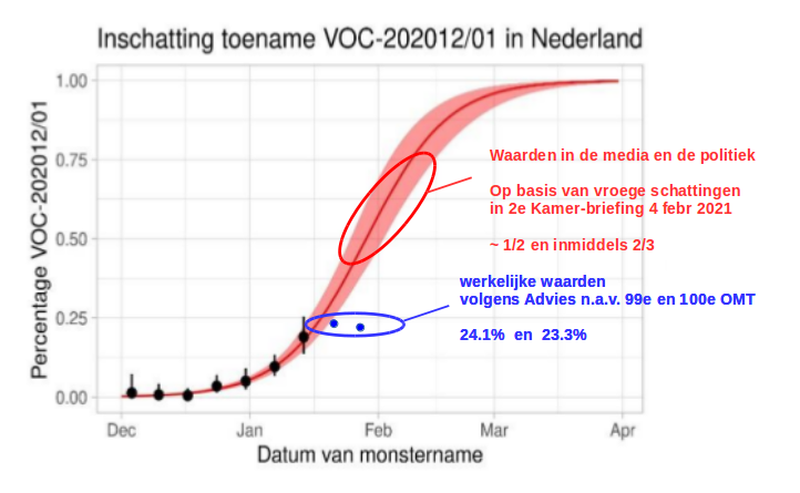
The "Mixed-Effects Models in S and S-PLUS" book by Pinheiro and Bates talks about non-linear mixed-effects models and gives a logistic model as an example to demonstrate the difference between linear and non-linear models.

$\>$$\>$$\>$ To illustrate these differences between linear and nonlinear models, let us consider a simple example in which the expected height $h_t$ of a tree at time $t$ follows a three-parameter logistic growth model. \begin{equation} h_t =\phi_1 / \{1 + \exp[- (t - \phi_2)/\phi_3 ]\}. \tag{6.1} \end{equation} As described in Appendix C.7, the parameters in (6.1) have a physical interpretation: $\phi_1$ is the asymptotic height; $\phi_2$ is the time at which the tree reaches half of its asymptotic height; and $\phi_3$ is the time elapsed between the tree reaching half and $1/(1 + e^{-1}) \simeq 3/4$ of its asymptotic height. The logistic model (6.1) is linear in one parameter, $\phi_1$, but nonlinear in $\phi_2$ and $\phi_3$.
$\>$$\>$$\>$ To make the example more concrete, suppose that $\phi_1 = 3$, $\phi_2 = 1$, and $\phi_3 = 1.2$ and that we initially want to model the tree growth for $0.4 \leq t \leq 1.6$. The logistic curve, shown as a solid line in Figure 6.1, is approximated very well in the interval $[0.4,1.6]$ by the fifth-degree polynomial \begin{equation} h_t \simeq -2.2911 + 16.591t - 44.411t^2 + 56.822t^3 - 31.514t^4 + 6.3028t^5 \end{equation} obtained as a least-squares fit to equally spaced $t$ values in the interval $[0.4,1.6]$. The polynomial fit, shown as a dashed line in Figure 6.1, is virtually indistinguishable from the logistic curve within this interval.
$\>$$\>$$\>$ Unlike the coefficients in the logistic model, the coefficients in the polynomial approximation do not have any physical interpretation. Also, the linear polynomial model uses twice as many parameters as the logistic model to give comparable fitted values. Finally, the polynomial approximation is unreliable outside the interval $[0.4,1.6]$. Figure 6.2, displaying the two curves over the extended interval $[0,2]$, shows the dramatic differences between the curves outside the original range. We would expect growth curves to follow a pattern more like the logistic model than like the polynomial model. (p.274)

I see the point of their explanation; however, one can also write that as a mixed-effect generalised linear model as something like

$logit(\boldsymbol{Y}) = \beta \boldsymbol{X} + \boldsymbol{b} + \epsilon$

Which would technically be a linear model?

Is this just semantics, or is there something more I am missing?

Answer 1

Short

For the sake of the point of the book, you can interpret 'linear function' in the narrow sense as a polynomial function, or as ordinary least squares regression.

It is not about the semantics of what is or what is not a linear model. In this case the example is not a GLM (more about that below), but that is besides the point. Even if it would be GLM then it would be different from a polynomial function and the parameters $\phi_2$ and $\phi_3$ would have meaningful physical interpretations.

More than semantics

As Gordon Smyth mentions in the comments, it is more than just semantics. Due to the parameter $\phi_1$ the logistic growth model is not exactly equal to the logistic function used in logistic regression.

Compare

$$\phi_1/\lbrace 1+\text{exp}[-(t-\phi_2)/\phi_3]\rbrace$$

with

$$1/\lbrace 1+\text{exp}[-(t-\phi_2)/\phi_3]\rbrace$$

Logistic regression and fractions

Logistic regression deals with $\phi_1=1$. This relates to fractions between zero and one. The example from the book is a growth model and a different setting.

Not all fractions are logistic regression

Sidenote: I am saying that logistic regression relates to fractions, but not all fractions relate to logistic regression.

When we deal with fractions then we still might have $\phi_1 \neq 1$ for instance the fraction of coronavirus variants relates to growth models, and has been modeled by some with logistic curves that wrongly assume $\phi_1 = 1$.

An example is the forecasting of variants by the Dutch 'RijksInstituut Voor Veiligheid (RIVM)'. Besides problems with the exponential growth of the two different strains (leading to large discrepancies in the odds far beyond the prediction intervals) the model wrongly assumed $\phi_1 = 1$. In the picture below we see that this has the effect of unrealistic predictions for April, with statements that the fraction of infections with the variant is gonna be close to 1 with a very tiny error margin (the reality is that it is currently somewhere in the range 0.8 to 0.9).

For the growth model we can come up with ideas why the $\phi_1$ should not be equal to 1. Also for other models that deal with fractions it might be wrong as well. This is in particular problematic when the curves are fitted based on little data in a small range and subsequently extrapolated. This may contribute, for instance, to the piranha problem. Assuming linearity/addition of multiple effects on the log-odds can be problematic.

---

The semantics

What is a linear model?

Linearity is a broad term.

One might for instance consider it a model that is a straight line $a+bx$ or more general a matrix equation $\beta X$. But linearity could also relate to a function with the algebraic property $f(x+y) = f(x) + f(y)$ and $f(a\cdot x) = a\cdot f(x)$.

In statistics we have linear regression which makes the predictor a weighted sum of the observations (a linear function of the observations).

$\hat\beta = M \cdot y$

For instance OLS with $M = (X^TX)^{-1}X^T$ or ridge regression with $M = (X^TX -\lambda I)^{-1}X^T$.

Generalized linear models (GLMs) are not like that. You can not find $\hat\beta$ as a sum of the observations $y$, and instead will use some itterative method to approach the solution. But still, there is a linear aspect to GLM, which is that transformation (by means of the link function) of the conditional expectation of the data is a linear function of the regressors.

So yes GLM is in one way linear, but in another way it is not.

---

The illustration

The point of the book seems to be different from the semantic point, and is more about the idea that the ubiquitous ordinary least squares (linear) model, like a polynomial, might gonna fit the data well, but is different in interpretation. The coefficients can be meaningless (if the model is not mechanistic/ab-initio) and you can not rely on extrapolation.

(You wrote that you got the point, but this is just to be complete and help other bystanders/readers)

• Polynomials, splines, with or without some transform (as in GLM), or other general curves... they are often used as an empirical model and they have the advantage of being easy to fit.

• Non-linear models, they are often a mechanistic model and they have the disadvantage of being less easy to fit (but they are still used because of the greater interpretability and also they might be used for extrapolation to some extent).

The problem with the point of the book is that sometimes a (generalized) linear model can be a mechanistic model. The point is not about the idea whether the growth curve is a linear function or not (in some way or another), but about the idea that polynomials are often standard fitting methods without mechanistic meaning. The idea is that a non-polynomial function could be better. And whether this non-polynomial function is a GLM model that can still be interpreted as linear, or a non-linear model, that is besides the point.

Answer 2

When log transforms are employed in function approximation, and

$\log(y)=\beta_0 + \beta_1x_{i1} + \beta_2x_{i2} + \cdots + \beta_j x_{ij}$

you will obviously have an arithmetic model that is "linear in the parameters." However, when looking at many of the non-linear Poisson regression models we use for fitting cancer incidence and mortality among atomic bomb survivors, the basic models are for example

$\lambda_{jk} =\exp\{\boldsymbol{\alpha}^T;\mathbf{x}\} \left[1+ \beta_k x_D \exp\{\beta_a x_{30} + \beta_t x_{70}\}\right], $

where the cancer rate in cell $jk$ of a multiway person-year tabulation table, $\lambda_{jk}$, cannot be linearized via the log-transform. Hence, in order to perform the regression one needs to take the first and second partial derivatives of $\lambda_{jk}$ w.r.t. $\alpha$ and $\beta$ coefficients and perform Newton-Raphson on the score vector and Hessian matrix in order to update parameters.

I don't see how you can shortcut the non-linear tree-growth model presented using only log transforms, since it's based on ratios and exponentials -- wholly non-linear. Also, if you think you can reduce a function via algebra and logarithms to its mostly linear form, it works out that the original first and second partial derivatives of coefficients that are within log/exp transforms will result in fastest convergence.

Answer 3

Pinheiro and Bates are comparing a logistic growth model to a linear combination of polynomials. Not a logistic regression. A logistic regression involves a single parameter p, which is then broken up into betas which are constants and are multiplied with x and all added together. That is a linear function. This logistic growth model has three parameters and the y is related to x (or t in this case) via a function that is nonlinear.

Of course, in logistic regression or all GLMs, there is a brief detour of requiring a link function to make the relationship between y and x linear. So strictly speaking, some function of y equals XB, but most people focus on the beta and because that is linear, or, to put it another way, x is linear in the logit scale so they call logistic regression linear.

So, in that sense, I think you’re right it is just a matter of semantics, but I don’t think this precludes what Pinheiro and Bates are talking about. If you read further down the book, they start talking about non-linear regression and again the expected value of y is equal to some non-linear function of x (equation 6.2 for example). Not y equals XB, or some function of y equals XB.