Interpreting coefficient changes in Cox PH model involving interactions

Question

I read the relevant questions here involving interactions in CoxPH (including 1, 2, 3, 4, 5, 6), and the relevant chapter of Applied Regression Analysis and Generalized Linear Models textbook. However, my confusion still persists about how to interpret interaction terms in CoxPH.

Particularly, my question is about 1) How to think about changing directions of hazard (good turning to bad) when interactions are present 2) How to interpret interaction coefficients involving two continuous predictor variables.

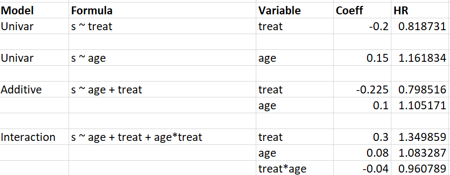
Let me demostrate it more concretely by providing two mock analyses below. The first case involves two variables age (continuous) and treat (dichotomous) variables; a simple model to examine how treatment and age affect survival. The results are below:

Please correct me if I'm wrong, but, I interpret the models as:

• (Univariate) Without taking age into account, the treatment reduces risk by 19% (1-0.81).
• (Univariate) Without taking treatment into account, each year passing (1 unit increase in age), the risk is increased by 16% (1.16-1).
• (Additive) When age is held constant (at every age value in the dataframe), treatment reduces risk by 21% (1-0.79). This assumes that there is no interaction between terms (ie. parallel slopes in the age vs outcome regression line fitted onto treatment or no treatment data subsets -- similar to Fig 7.4 in the book I mentioned earlier ).
• (Additive) , Each passing year, the risk is increased by 10% (1.10-1), in both treatment and no treatment groups. The lower hazard ratio for age in additive model may suggest, with treatment the negative effect of aging is diminished.
• (Interaction) This is where it gets confusing for me: How to interpret a higher risk calculated for the treat variable here, while it was associated with lower risk previously? Does that mean, the treatment is actually bad for certain age groups? Also what to make of the HR value lower than 1 for the interaction term? I guess I'm looking for an intuitive explanation of the situation here.

The second case involves interaction between two continuous variables. Analysis from real world data gave me the following parameters:

Here, Gene1 seems to be "bad" (ie high risk), and Gene2 is good (ie low risk) although Gene2 is not significant. In the interaction model, all the regressors were found significant, and the interaction term provides the highest risk of all. Is the following a proper interpretation of this data?

• (Additive) Each unit increase in Gene1 is associated with 23% increase in risk (holding Gene2 constant)
• (Additive) Each unit increase in Gene2 is associated with 10% decrease in risk (holding Gene1 constant)
• (Interaction) Again, it gets tricky here: A simultaneous 1 unit increase in both Gene1 and Gene2 leads to %37 increase in risk (?). Biologically this might mean that the increase in the "bad" gene expression overrides the increase in "good" gene expression, resulting in a higher risk (?).
• (Interaction) How to think about the coefficients/HR values of Gene1 (17% increase in risk) and Gene2 (17% decrease in risk) in and of itself in the context of the said interaction.

I hope I'm not missing a crucial point here. Any insight is appreciated.

Answer 1

That is exceptionally well laid out. As I detail in RMS it is not so fruitful to emphasize individual coefficient interpretation except for the highest-order term. That is, the interaction term can be interpreted (especially when one of the interacting variables is binary) but lower order terms (often called "main effects" but this is a bit misleading) are heavily depending on centering and indicator variable coding. Think instead of contrasts, which are most easily calculated in terms of differences in predicted values (here, differences in log relative hazard, so that the anti-log of the contrast is a hazard ratio).

What I'm about to describe doesn't work as well if any of the effects is nonlinear. In that case the choice of intervals is arbitrary and can even be misleading if there is a flat or non-monotonic piece of one of the covariate effects. Supposing effects are linear (which has to be the case for binary predictors), suppose you want to estimate the effect of x1 where x1 interacts with x2. Pick a series of values of x2. For each x2 contrast the relative log hazard when x1 is set to a vs. when x1 is set to b. For binary x1, a=0, b=1. For continuous x1 you might let a=first quartile of x1, b=upper quartile of x1.

In the R rms package the contrast function (long name contrast.rms) makes contrasts over a series of x2 values very easy to do no matter how complex the model. When getting differences in predicted values one can easily compute the standard error of each difference, as contrast does.

As shown in the RMS course notes, for the continuous-continuous x1 x2 case it works well to graph a color image plot where the 'temperature' of the the color represents the log hazard or survival probability.

If you evaluate any of the contrasts manually you'll see that the x1 effect is a simple function of x2. And as you referenced, large negative interaction terms can lead to reversals of x1 effects as x2 changes.

Note that the univariable estimates you provided are not helpful.