Calculate certainty of Monte Carlo simulation

Question

(Hi, sorry, this is probably a very entry level question for this site. Let me know if something is not OK.)

Let's say that we use the Monte Carlo method to estimate the area of an object, in the exact same way you'd use it to estimate the value of π.

Now, let's say we want to calculate the certainty of our simulation result. We've cast n samples (taken from uniform distribution of the sample area), m of which landed inside the object, so the area of the object is approximately m/n of the total sampled area. We would like to make a statement such as:

"We are 99% certain that the area of the object is between a₁ and a₂."

How can we calculate a₁ and a₂ above (given n, m, total area, and the desired certainty)?

I wrote a program which attempts to estimate this bound numerically. Here the samples are points in [0,1), and the object is the segment [0.25,0.75). It prints a₁ and a₂ for 50%, 90%, and 99%, for a range of sample counts:

import std.algorithm;
import std.random;
import std.range;
import std.stdio;

void main()
{
    foreach (numSamples; iota(0, 1000+1, 100).filter!(n => n > 0))
    {
        auto samples = new double[numSamples];
        enum objectStart = 0.25;
        enum objectEnd   = 0.75;

        enum numTotalSamples = 10_000_000;
        auto numSizes = numTotalSamples / numSamples;
        auto sizes = new double[numSizes];
        foreach (ref size; sizes)
        {
            size_t numHits;
            foreach (i; 0 .. numSamples)
            {
                auto sample = uniform01!double;
                if (sample >= objectStart && sample < objectEnd)
                    numHits++;
            }

            size = 1.0 / numSamples * numHits;
        }

        sizes.sort;
        writef("%d samples:", numSamples);
        foreach (certainty; [50, 90, 99])
        {
            auto centerDist = numSizes * certainty / 100 / 2;
            auto startPos = numSizes / 2 - centerDist;
            auto endPos   = numSizes / 2 + centerDist;
            writef("\t%.5f..%.5f", sizes[startPos], sizes[endPos]);
        }
        writeln;
    }
}

(Run it online.) It outputs:

//                     50%                 90%                 99%
100 samples:    0.47000..0.53000    0.42000..0.58000    0.37000..0.63000
200 samples:    0.47500..0.52500    0.44500..0.56000    0.41000..0.59000
300 samples:    0.48000..0.52000    0.45333..0.54667    0.42667..0.57333
400 samples:    0.48250..0.51750    0.46000..0.54250    0.43500..0.56500
500 samples:    0.48600..0.51600    0.46400..0.53800    0.44200..0.55800
600 samples:    0.48667..0.51333    0.46667..0.53333    0.44833..0.55167
700 samples:    0.48714..0.51286    0.46857..0.53143    0.45000..0.54857
800 samples:    0.48750..0.51250    0.47125..0.53000    0.45375..0.54625
900 samples:    0.48889..0.51111    0.47222..0.52667    0.45778..0.54111
1000 samples:   0.48900..0.51000    0.47400..0.52500    0.45800..0.53900

Is it possible to calculate these numbers directly instead?

(Context: I'd like to add something like "±X.Y GB with 99% certainty" to btdu)

Answer 1

Consider the following Monte Carlo approximation in R of $P(.25 \le U < .75) = 0.5,$ for $U\sim\mathsf{Unif}(0,1).$

set.seed(2021)                 # for reproducibility 
u = runif(10^6)                # 10^6 - vector of std unif values
event = (u >= .25)&(u < .75)   # logical 10^6 - vector
mean(event)                    # proportion of TRUEs
[1] 0.500772
1.96*sd(event)/10^3            # aprx 95% margin of simulation error
[1] 0.0009799993

The Law of Large Numbers guarantees the approach of the approximated value to the exact value $1/2$ as the number of iterations increases to infinity. In our particular case, we can use a well-known Wald asymptotic 95% confidence interval to find the approximate margin of simulation error. Specifically, for the $B = 10^6$ iterations shown, the margin of simulation error is about $0.00098$ so we can say with 95% confidence that the desired probability is $0.5008 \pm 0.0010.$

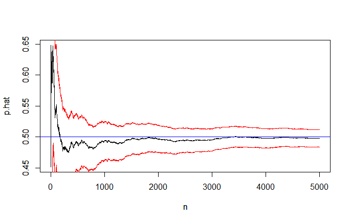
Here is a plot of estimated proportions p.hat(black) and corresponding Wald 95% CIs after each of the first 5000 of the million iterations. (CI's for $n < 1000$ should be taken as rough approximations.)

n = 1:5000
p.hat = cumsum(u[1:5000])/n
plot(n, p.hat, type="l")
 abline(h=.5, col="blue")
Up = p.hat + 1.96*sqrt(p.hat*(1-p.hat)/n)
Lw = p.hat - 1.96*sqrt(p.hat*(1-p.hat)/n)
 lines(Up, type="l", col="red")
 lines(Lw, type="l", col="red")

Addendum (per @whubers's Comments below): For large $n,$ say $n \ge 1000,$ the Wald intervals (illustrated in the figure above show that the estimate, $\hat p = X/n$ is near to $p = 1/2.$ So without simulation, one would have the 95% CI $\hat p \pm 1.96\sqrt{\frac{\hat p(1-\hat p)}{n}}$ for $p = 1/2.$ [These are the intervals for $n=1,2, \dots, 5000$ shown in red in the figure.] For smaller $n,$ a more accurate 95% Agresti-Coull CI uses point estimate $\check p = \frac{X+2}{n+4}$ to make the interval $\check p \pm 1.96\sqrt{\frac{\check p(1-\check p)}{n+4}}$ (not shown in the figure).

Notes:

(1) We assume that R code runif gives values that cannot, for practical purposes, be distinguished from IID standard uniform observations.

(2) Computer code should be commented.

(3) For reproducibility, the seed should be shown for a simulation.

(4) event is a logical vector of one million TRUEs and FALSEs; its 'mean' is the proportion of its TRUEs. [TRUE is taken as 1, and FALSE as 0; similarly for sd.]

(5) The Wald 95% asymptotic CI for a binomial proprotion is $\hat p \pm 1.96\sqrt{\frac{\hat p(1-\hat p)}{n}},$ where $X$ successes are observed among $n$ trials and $\hat p = X/n.$