Why are extreme correlations so common in this Monte Carlo simulation? [duplicate]

Question

Consider the following simple Monte Carlo:

import matplotlib.pyplot as plt
import numpy as np
from scipy.stats import pearsonr
r = np.arange(3)+1
R = [pearsonr(np.random.normal(0,1,3), r)[0] for i in range(5009)]
plt.hist(R, bins=100)
plt.xlabel('Pearson\'s Correlation Coefficient')
plt.ylabel('Frequency')
plt.show()

Which gives a diagram similar to the following:

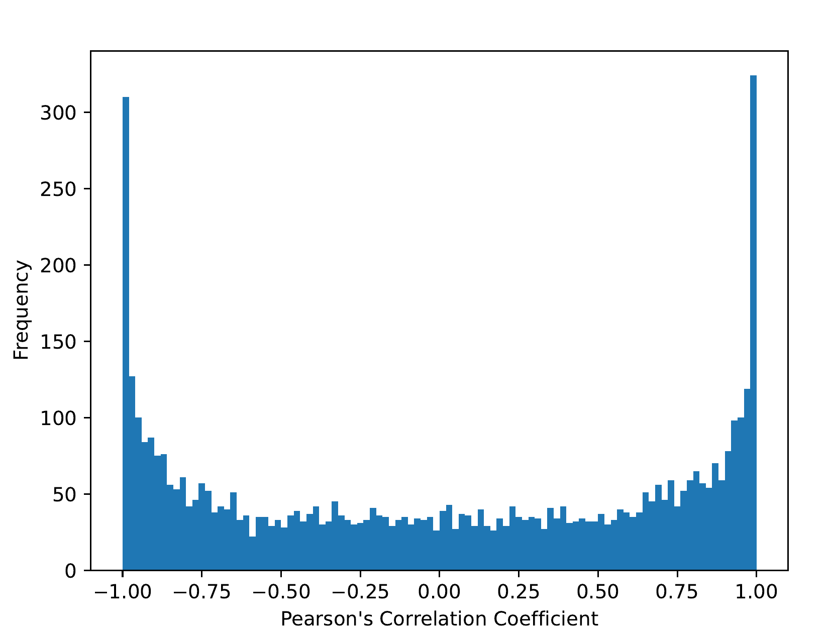
In words, 5009 IID standard normal variables are sampled in triplicate (n=3) and are paired to the values (1,2,3). The code above computes the Pearson's product-moment correlation coefficient between the triplicate standard normal variable measures and the sequence (1,2,3). I am curious about the distribution that results, which appears to my surprise to be non-uniform. I suspect there is a mathematical reason behind this reproducible effect.

Is there a mathematically formal reason why the extreme correlations of $\pm 1$ are more common than the less extreme correlation scores?

Answer 1

Is there a mathematically formal reason why the extreme correlations of ±1 are more common than the less extreme correlation scores?

COOLSerdash gives in the comments the exact distribution of the sample distribution of the correlation coefficient. But this does not directly answer why we get so often values close to the extremes.

---

Intuition in terms of geometry of fitting

For an intuition why the correlation is so extreme you might consider the distribution of $R^2$.

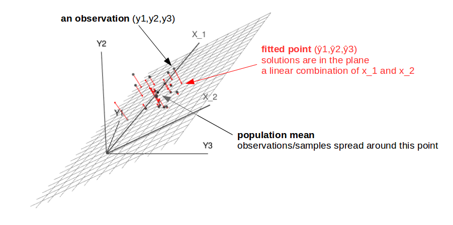
You can regard correlation as a linear fit which splits the random variable $y$ into a linear model part and a noise part. This has a geometric interpretation of a perpendicular projection of the n-dimensional datapoonts $y$ onto a surface spanned by two vectors $a \cdot \vec{1} + b \vec{x}$. See for instance the illustration from this question

The value of $R^2$ is the ratio of the variance in these two components, the ratio of the variance in the model part and the variance in the total.

The variance of these model and noise components (which, by the way, are independent) are $\chi^2(\nu)$ distributed with the model part one degree of freedom $\nu=1$ and the noise $\nu=n-2$ degrees of freedom. So the distribution of $R^2$ is similar to

$$\frac{X_{model}}{X_{noise} + X_{model}} \quad \text{with $X_{model} \sim \chi^2(1)$ and $X_{noise} \sim \chi^2(n-2)$}$$

when $X_{noise}$ is small this ratio is relatively more often close to $1$.

We can also express $$1/R^2 = 1 + \frac{X_{noise}}{X_{model}}$$

which is similar to a F-distributed variable shifted by 1. When the degrees of freedom in the noise are low then this $1 + \frac{X_{noise}}{X_{model}}$ will be close to 1.

Answer 2

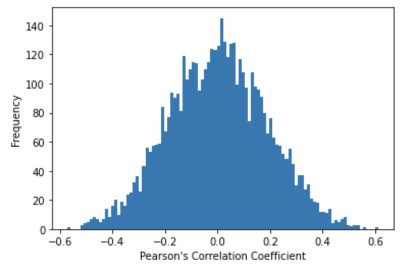
Vector length seems to be too small, $n$, trying $30$. Minor changes to your sample code:

import matplotlib.pyplot as plt
import numpy as np
from scipy.stats import pearsonr
r = np.arange(30)+1
R = [pearsonr(np.random.normal(0,1,30), r)[0] for i in range(5009)]
plt.hist(R,bins=100)
plt.xlabel('Pearson\'s Correlation Coefficient')
plt.ylabel('Frequency')
plt.show()

Also, if we think that a noise should be uncorrelated, so correlations should look like normal centred at zero, not uniform:. This is the consequence of law of large numbers, intuitively.

Edit: Good point from @user20160. The length argument can be thought in terms of Autocorrelation Functions in time-series. Because observation is valid for two random variates too. So increasing length will decrease ACF to 0, mean value in the simulation. For small n=2, it is all fully correlated then it decays with increasing length.