There are several methods in common use. I will discuss a few. I suppose none of them is perfect. However, each of them is sometimes helpful.
(1) Physical laws. Example: For a radioactive substance with a long half life, the waiting time between particle emissions will not change much during a lab experiment of several weeks. In some cases, there are good theoretical reasons to suppose that the
waiting times are exponential.
(2) Supposed source of the data. Test scores are
often sums or averages of many equally weighted questions. Then the Central Limit Theorem suggests
that the scores should be approximately normal.
If these are standardized nationwide tests, then
the companies making the tests may have 'tweaked'
the test so that scores turn out to be even closer
to normal than would be the case just from the CLT.
(They may delete questions that get unpredicted answers, or include new questions that have been pre-tested
to give sensible results.)
Also, heights of people can be viewed as sums of various body parts. Although not independent and identically distributed, these terms may lead to approximately
normal heights In practice, heights are often mixtures of normal distributions with means not many standard deviations apart, and thus still approximately normal.
(Mixtures of ages, genders, ethnicities, etc.)
(3) Traditional practice. Sizes of bank accounts may follow Pareto distributions. Maybe less often than
supposed, but there is some variety among Pareto distributions and so some Pareto distribution may work pretty well---even if not perfectly. And it might take a lot of explaining why one wants to use something nontraditional.
In queueing theory, it is routinely assumed that service times are exponentially distributed. Because of the no-memory property of exponential distributions, the math is easier to handle with
exponential distributions. Consequently, the wait
of a customer standing in line for service is
taken to be the sum of exponential waiting times and thus gamma (or Erlang) distributed. (Exponential distributions are mathematically simple, and so IMHO often used in
a triumph of simplicity over accuracy.)
Lifetimes of components and assemblies of components are sometimes modeled using Weibull
distributions--especially when the failure rate
changes over time so that exponential models do not work.
(4) Distribution-finding software procedures. Many statistical software programs (R, Minitab, and many others) have procedures that take large samples and suggest
what distributions they might follow. You have
to use the output with care: some distribution families overlap (exponential, gamma, Weibull, etc.) Because of anomalies of a particular sample a more complicated family may be chosen as fitting
best, while a simpler one may fit almost as well,
be easier to use, and ultimately turn out to be right.
(5) Goodness of fit tests. If you suspect that data
are normal and have a few thousand observations,
you might try a Shapiro-Wilk GOF test to see if
your suspicions have validity. In for the sample
below (generated as normal), it is no surprise
that that the S-W P-value is large, suggesting
that the data are consistent with a normal distribution.
set.seed(2022)
x = rnorm(1000, 50, 7)
shapiro.test(x)

        Shapiro-Wilk normality test

data:  x
W = 0.99812, p-value = 0.3351
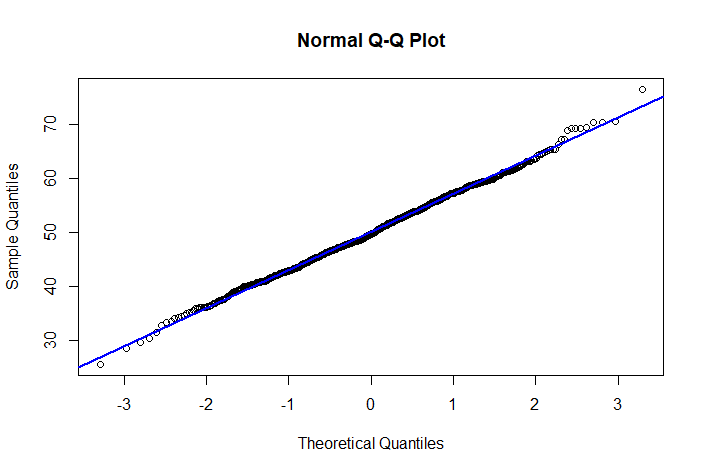
One might also use a normal probability plot (quantile-quantile plot),
which should show points mostly along a straight
line for truly normal data (not being too fussy
about linearity near the right and left ends).
qqnorm(x); qqline(x, col="blue", lwd=2)

If you have a specific distribution in mind (including its parameters), you might use a
Kolmogorv-Smirnov test to see if the CDF of
the proposed distribution matches the empirical CDF (ECDF) of your sample. [Adjustments, not shown here, are necessary if you have to estimate parameters.]
set.seed(203)
y = rexp(1000)         # 1000 samples from exponential
ks.test(y, pnorm, 1,1) # you suspect NORM(1,1)

        One-sample Kolmogorov-Smirnov test

data:  y
D = 0.15886, p-value < 2.2e-16
alternative hypothesis: two-sided
The hunch that the data may be $\mathsf{Norm}(\mu=1,\sigma=1)$ is very strongly rejected with P-value very near $0.$
Here is a plot of the ECDF of the data along with
the CDF pf $\mathsf{Norm}(\mu=1,\sigma=1).$ The K_S test statistic $D$ is the maximum vertical discrepancy between the ECDF (black) and the CDF (red).
plot(ecdf(y))
curve(pnorm(x,1,1), add=T, col="red", lwd=2)
   # 'x' is mandatory part of syntax


