Comparing residuals in two regression models

Question

Let us have two linear models. Let $\alpha_i$ be real numbers same in both.

$$ LM1: Y=\alpha_0 + \alpha_1X_1+\alpha_2X_2 + \varepsilon $$

$$ LM2: Y^\prime=\alpha_0 + \alpha_1X^\prime_1+\alpha_2X^\prime_2 + \varepsilon` $$

The difference between them is only in the fact that $X_i, X^\prime_i$ are different. Now, I want to test a hypothesis that the noise distribution remains the same $H_0: \varepsilon\overset{D}{=}\varepsilon`$ (we assume noise has a zero mean and finite variance). We have available random samples, from the first one of length $n$: $(Y_1, X_1)^\top, \dots, (Y_{n}, X_{n})^\top$, and from the second one with length $m$: $(Y`_1, X`_1)^\top, \dots, (Y`_{m}, X`_{m})^\top$.

My approach: Based on these samples, we estimate $\hat{\alpha_i},\hat{\alpha_i}^\prime $ where e.g. $\hat{\alpha_i}^\prime$ is the estimation using LSE from the LM2. Now, compute the residuals. So $\hat{\varepsilon}=Y-\hat{\alpha_0}-\hat{\alpha_1}X_1 - \hat{\alpha_2}X_2$ and similarly for the second model $\hat{\varepsilon}^\prime$.

Asymptotically $\hat{\varepsilon}\overset{D}{=}\hat{\varepsilon}^\prime$, as $n,m\to\infty$ because estimates of the coefficients are consistent. BUT, for finite $n$, we did not converge yet to these limits. If I do e.g. KStest ($ks.test(rez1, rez2)$), it will reject this hypothesis too often even if it is true. Is it a correct test at least asymptotically? Do you know about some other test comparing these distributions with a proper $p-$ value?

My interest is more academic and I want a test that provably works.

Here is also some idea of the sample code I used

\documentclass{article}
\usepackage{listings}
\begin{document}

\begin{verbatim}

n=1e+04 f <- function(X1, X2){return(-1 + 1X1 + 2X2)}

X11=rnorm(n, 0,1);X12=rnorm(n, -1, 2) Y1= f(X11, X12) + rLaplace(n)

fit=lm(Y1~X11+X12, data= data.frame(Y1, X11, X12)) rez1=fit$residuals

X21=rexp(n, 1);X22=rexp(n,2) Y2= f(X21, X22) + rLaplace(n)

fit2=lm(Y2~X21+X22, data= data.frame(Y2, X21, X22)) rez2=fit2$residuals

ks.test(rez1, rez2))

\end{verbatim}

\end{document}

Answer 1

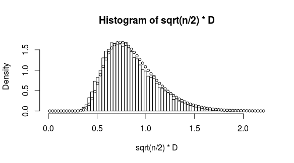
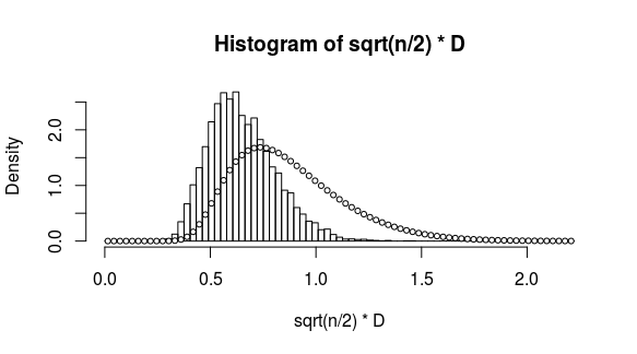
I can replicate the problem from the question with the code below. The discrepancy between the distribution of the test statistic and the Kolmogorov distribution can be changed by manipulating the fit. If we use an intercept lm(Y~1+X1+X2)$residuals then the difference is largest.

• Without intercept, the difference is only small

• With intercept, the difference is large

The case with only an intercept

We get the discrepancy already when we use only an intercept, ie. if we would model lm(Y~1)$residuals.

The discrepancy due to the intercept is easier to understand. The sampling of residuals is not independently drawing from a distribution for the residuals. Instead, the residuals will be correlated (the same is true for the case without intercept, but less strong).

This is most easy to see for the case of a sample of size 2 that is being modeled by only an intercept. The residuals will equal $\pm |x_1-x_2|$ and are symmetric.

More generally, for larger $n$, the residuals can be equated as

$$r_i = \epsilon_i - \frac{1}{n} \sum_{j=1}^n \epsilon_j $$

This makes the residuals multivariate normal distributed, if the $\epsilon$ are normal distributed. If we consider $\epsilon \sim N(0,1)$ then the covariance matrix for the $r_i$ is

$$ \Sigma_{ij} = \begin{cases} \frac{(n-1)^2}{n^2} & \quad \text{if $i=j$}\\ -\frac{n-1}{n^2} & \quad \text{if $i \neq j$} \end{cases} $$

We can obtain the same result by sampling from a multivariate normal distribution with this correlation. In the code below we did this with the function sim2 which produces the following image

Intuitively, what's happening?

The Kolmogornov Smirnoff test compares the deviation of the empirical distribution function. Let's focus on this distribution in a single point, at zero.

The error terms, if they are distributed as a standard normal distribution, then they will have fifty-fifty probability to be above or below the point zero. The empirical distribution in the point zero will follow a binomial distribution with $n$ trials and $p=0.5$.

The residual terms will be different. The residual terms are transformed error terms.

The fit with an intercept will shift the terms up or down. If there are many error terms above zero then a mean above zero is more likely and a shift down will be more likely. If there are many error terms below zero then a mean below zero is more likely and a shift up will be more likely.

So in comparison to the error terms, the residual terms will have a smaller variation for the empirical distribution in the point zero.

R-code

### function to simulate data 
### and compute test statistic for KS test
sim = function(n = 100, plot = "n") {
  X1 = rnorm(n)
  X2 = rnorm(n)
  Y = rnorm(n) 
  R1 = lm(Y~0+X1+X2)$residuals

  # use these alternatives below to get the clearest discrepancy
  #R1 = lm(Y~1+X1+X2)$residuals
  #R1 = lm(Y~1)$residuals

  X1 = rnorm(n)
  X2 = rnorm(n)
  Y = rnorm(n) 
  R2 = lm(Y~0+X1+X2)$residuals

  # use these alternatives below to get the clearest discrepancy
  #R2 = lm(Y~1+X1+X2)$residuals
  #R2 = lm(Y~1)$residuals
  
  if (plot == "y") {
    plot(R1[order(R1)],1:n, type ="l")
    lines(R2[order(R2)],1:n, col = 2)
  }
  test = ks.test(R1,R2)
  return(test$statistic)
}



### function to simulate data using multivariate normal
sim2 = function(n = 100, plot = "n") {
  ### create covariance matrix for mvrnorm distribution
  Sig = matrix(-(n-1)/n^2,n,n)
  diag(Sig) <- rep((n-1)^2/n^2,n)
  
  R1 = MASS::mvrnorm(1, mu = rep(0,n), Sigma = Sig)
  R2 = MASS::mvrnorm(1, mu = rep(0,n), Sigma = Sig)
  
  if (plot == "y") {
    plot(R1[order(R1)],1:n, type ="l")
    lines(R2[order(R2)],1:n, col = 2)
  }
  test = ks.test(R1,R2)
  return(test$statistic)
}

### perform 10^3 simulations and plot histogram
set.seed(1)
n = 600
D = replicate(10^4,sim(n))

br = seq(0,max(D)+d,1/n)*sqrt(n/2)
hist(sqrt(n/2)*D, breaks = br, freq = 0)

### function to compute kolmogorov distribution
pkolm = function(x) {
  k = 1:100
  sqrt(2*pi)/x*sum( exp(-(2*k-1)^2*pi^2/(8*x^2)) )
}
pkolm = Vectorize(pkolm)

### add kolmogorov distribution to histogram
P = c(pkolm(br))
P[1] = 0
points(br[-1]-br[2]/2, diff(P)/br[2])