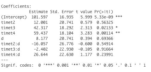
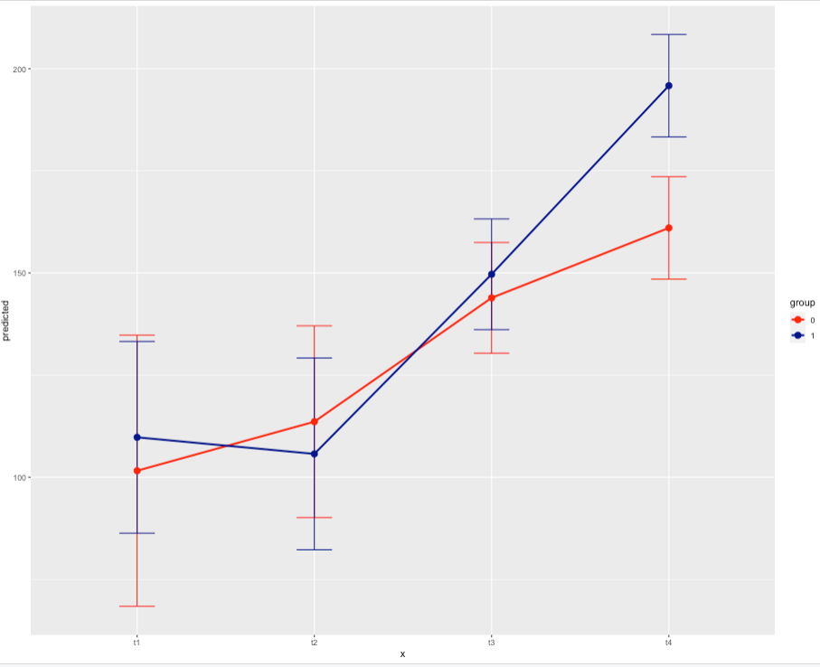
the interaction is significant as shown in the Figure below but is not in the regression table.
The regression table by itself does not represent the significance of a multi-level categorical predictor. That's the case whether there's an interaction or not.
The "significance" of the individual interaction coefficients represents whether each of them is individually different from a value of 0. That doesn't, however, examine whether the interaction term as a whole is significant. For that you need something beyond the coefficient table.
You can see the source of confusion by simply resetting the reference level for the categorical predictor time.
df$time<-factor(df$time)
df2<-df
df2$time <- relevel(df2$time,ref="t4")
model2 <- lm(y~time*d,data=df2)
summary(model2)
## extract to match what's shown in OP
## Coefficients:
##             Estimate Std. Error t value Pr(>|t|)
## (Intercept)  161.033      6.401  25.158  < 2e-16 ***
## timet1       -59.437     18.104  -3.283 0.001140 **
## timet2       -47.435     13.578  -3.494 0.000543 ***
## timet3       -17.120      9.422  -1.817 0.070140 .
## d             34.821      9.052   3.847 0.000144 ***
## timet1:d     -26.644     22.630  -1.177 0.239910
## timet2:d     -42.702     19.202  -2.224 0.026856 *
## timet3:d     -29.046     13.324  -2.180 0.029985 *
ALL of the coefficient estimates including the intercept have been changed from the model in the question. Two of the interaction coefficients are now "significant" by the p < 0.05 criterion.
Yet all we have done is change the reference level of one categorical predictor.
If a predictor is involved in an interaction, its "main effect" coefficient estimate (with default treatment/dummy coding) is for the situation when all its interacting predictors are at 0 (continuous predictors) or the reference level (categorical predictors). That principle extends to the intercept and to interaction terms involving multi-category predictors, too.*
Re-centering/re-ordering one predictor will affect the regression coefficient estimates of any other predictors with which it interacts. That's frequently overlooked and a massive source of confusion, base on how many such questions we see on this site.
The two models are functionally identical, as one should expect. Predictions take into account the model-specific coefficient estimates and their covariances so that predictions for any particular choice of predictor values are the same. Here are predictions for all 8 combinations of time and d, from both models.
 predict(model,data.frame(time=rep(c("t1","t2","t3","t4"),2),d=rep(c(0,1),times=c(4,4))))
##        1        2        3        4        5        6        7        8
## 101.5968 113.5979 143.9137 161.0333 109.7737 105.7174 149.6889 195.8546
 predict(model2,data.frame(time=rep(c("t1","t2","t3","t4"),2),d=rep(c(0,1),times=c(4,4))))
##        1        2        3        4        5        6        7        8
## 101.5968 113.5979 143.9137 161.0333 109.7737 105.7174 149.6889 195.8546
The models have identical overall significance, as shown by anova()
anova(model)
## Analysis of Variance Table
##
## Response: y
##            Df Sum Sq Mean Sq F value    Pr(>F)
## time        3 233474   77825 27.1367 1.133e-15 ***
## d           1  22906   22906  7.9870  0.005006 **
## time:d      3  21600    7200  2.5106  0.058686 .
## Residuals 322 923458    2868

anova(model2)
## Analysis of Variance Table
##
## Response: y
##            Df Sum Sq Mean Sq F value    Pr(>F)
## time        3 233474   77825 27.1367 1.133e-15 ***
## d           1  22906   22906  7.9870  0.005006 **
## time:d      3  21600    7200  2.5106  0.058686 .
## Residuals 322 923458    2868
Note that in these simulated data the overall interaction coefficient isn't quite "significant" by the usual arbitrary p < 0.05 criterion. If there were particular pre-specified combinations of time and d of interest, however, you could make those comparisons without worrying about the lack of "significance."
This page shows how to use a likelihood-ratio test between 2 models to examine the overall significance of a multi-category predictor. The same principle applies here with the interaction: compare the models with and without the interaction term to get the best estimate of the overall "significance" of the interaction.
modelAdditive <- lm(y~time+d,data=df)
anova(modelAdditive,model)
## Analysis of Variance Table
##
## Model 1: y ~ time + d
## Model 2: y ~ time * d
##   Res.Df    RSS Df Sum of Sq      F  Pr(>F)
## 1    325 945058
## 2    322 923458  3     21600 2.5106 0.05869 .
In this case the result is the same as seen for the interaction term in the single model. With multiple interactions or levels of interactions, however, the problems with the type of ANOVA and the listed order of variables can lead to further confusion.
This page illustrates a "chunk test" approach, tests that examine all coefficients involving each set of predictors/interactions together. That's a very general approach that doesn't require re-fitting the model and directly evaluates all non-linear terms and interactions in the model. It's implemented in the anova() function that's specific to models generated by the rms package in R.
library(rms)
modelOLS = ols(y~time*d, df)
anova(modelOLS)
##                 Analysis of Variance          Response: y
##
##  Factor                                  d.f. Partial SS MS        F     P
##  time  (Factor+Higher Order Factors)       6  262146.28  43691.047 15.23 <.0001
##   All Interactions                         3   21600.10   7200.034  2.51 0.0587
##  d  (Factor+Higher Order Factors)          4   44505.75  11126.437  3.88 0.0043
##   All Interactions                         3   21600.10   7200.034  2.51 0.0587
##  time * d  (Factor+Higher Order Factors)   3   21600.10   7200.034  2.51 0.0587
##  REGRESSION                                7  277980.02  39711.432 13.85 <.0001
##  ERROR                                   322  923458.15   2867.882
In my experience the "chunk" tests are least likely to lead to confusion with more complicated models, particularly those that go beyond ordinary least squares.
*An interaction coefficient under treatment/dummy coding represents the difference from what might have been predicted based solely on the intercept, "main effects," and lower-level interactions. All those are changed in model2 from model. Note that the timet1:d coefficient in model2 is the negative of the timet4:d coefficient in model. That's because the reference roles of timet1 and timet4 have switched between the two model.


