3
$\begingroup$

I use the generalized form of the Student's-t distribution: \begin{align*} f(l|\nu ,\mu ,\beta) = \frac{\Gamma (\frac{\nu+1}{2})}{\Gamma (\frac{\nu}{2}) \sqrt{\pi \nu} \beta} \left(1+\frac{1}{\nu}\left(\frac{l - \mu}{\beta}\right)^2 \right)^{\text{$-\frac{1+\nu}{2}$}} \end{align*}

I want to have standardized version, i.e. mean zero and a variance of one. Therefore, I set $\mu=0$ and \begin{align*} \beta=\sqrt{\frac{\nu-2}{\nu}} \end{align*} which ensures, that the variance is equal to one. If I now insert this I get after some derivations \begin{align*} f(l|\nu) =(\pi (\nu-2))^{-\frac{1}{2}}\Gamma \left(\frac{\nu}{2} \right)^{-1} \Gamma \left(\frac{\nu+1}{2} \right) \left(1+\frac{l^2}{\nu-2} \right)^{-\frac{1+\nu}{2}} \end{align*} Now my question is: What is the formula for the kurtosis? Is it still $\frac{6}{\nu-4}$?

E.g. consider these data and the following R code:

pinumber<-3.141592653589793
startvalue<-2

loglikstandardizedt <-function(par){
if(par>0) return(-sum(log((pinumber*(par-2))^(-1/2)*gamma(par/2)^(-1)*gamma((par+1)/2)*(1+standresidsapewma^2/(par-2))^(-(1+par)/2))))
else return(Inf)
}

optim(startvalue, fn=loglikstandardizedt, method="Brent",lower=2,upper=250)
param = optim(startvalue,loglikstandardizedt, method="BFGS")$par

If I look at the plot, to see how good the fit is, I do the following code:

 # control output
    denstiystandtresid<-function (x) (pinumber*(param-2))^(-1/2)*gamma(param/2)^(-1)*gamma((param+1)/2)*(1+x^2/(param-2))^(-(1+param)/2)

    plot(density(standresidsapewma),ylim=c(0,0.8))
    curve(denstiystandtresid,col="red",add=TRUE)

This gives me the following plot: plotgraph
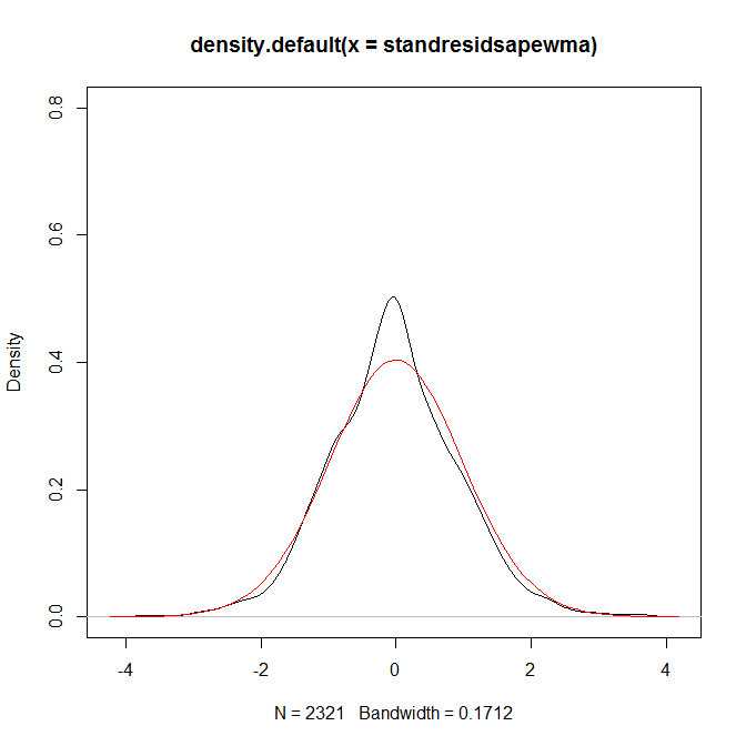
As you can see, the fit is, let's say fairly ok. Now, I am interested in the excess kurtosis. The data has the excess kurtosis of

kurtosis(standresidsapewma)

which gives 0.6470055

I would expect, since the fit is quite ok in the tails, that the fitted distribution has almost the same excess kurtosis, but if I calculated it via the following way (the estimate output for $\nu$ is 8.85009):

$\frac{6}{\nu-4}=\frac{6}{8.85009-4}=1.23709$?

which is pretty much more than 0.64. This seems to be wrong to me, since I believe, that the fit in the tail is quite ok, so the kurtosis should be almost the same? Is my formula for calculating the ex kurtosis in case of a standardized Student's-t distribution wrong? Or what is my mistake?

$\endgroup$
1
  • 2
    $\begingroup$ Kurtosis by definition is invariant under affine linear transformations, which includes standardization. That fit is pretty bad, by the way: using a histogram-like presentation only obscures the differences. $\endgroup$
    – whuber
    Commented Apr 25, 2013 at 13:17

2 Answers 2

4
$\begingroup$

Sample moments typically converge slowly to the true moments. This is the reason why you are observing such discrepancies between the two methods. For instance, run the following code several times

# Simulated data
dat <- rt(2000,df=8)

# Sample kurtosis
kurtosis(dat)-3

# Theoretical kurtosis
6/(8-4)

# MLE kurtosis
LL <- function(par){
if(par>0) return(-sum(dt(dat,df=par,log=T)))
 else return(Inf)
 }

 parameter <-optim(8, fn=LL, method="Brent",lower=6,upper=11)$par

6/(parameter-4)

In many cases the two estimators (sample kurtosis and MLE) differ. You got one of those samples where they differ.

Moreover (and maybe more importantly), the sample kurtosis converges to the true kurtosis while the MLE kurtosis converges to the kurtosis of the distribution that better fits the true distribution according to this criterion.

I agree with @whuber that the fit of your proposal distribution is pretty bad. You are unnecesarilly restricting the distribution (a Student-t would provide a much better fit for almost the same computational cost). Check

 library(MASS)
 fitdistr(standresidsapewma,"t")
$\endgroup$
2
$\begingroup$

Kurtosis does not just measure tail heaviness. It also measures peakedness. A distribution that is similar in the tails but more peaked will tend to have higher kurtosis than one that is less peaked.

Another way to think of kurtosis is as follows:

Define the 'shoulders' of a density as being at $\mu \pm \sigma$. Then the kurtosis can be thought of as (a constant plus) the square of the variabliity about the shoulders. That is, the more the probability moves away from the shoulders, the bigger the kurtosis tends to become.

This broad tendency is not a theorem by any means; it's possible to arrange to move the probability around in such a way that the peak increases while the kurtosis goes down. [The issue comes down to how you define "similar in the tails".]

See the first paragraph here:

http://en.wikipedia.org/wiki/Kurtosis

$\endgroup$
3
  • $\begingroup$ This is not mathematically correct, Glen_b. Kurtosis measures virtually nothing about peakedness, and also nothing about probability content within the shoulders. The contribution of the peak to the kurtosis statistic is minimal as I have shown in my TAS paper. Instead, kurtosis measures tails, for all practical purposes. There are no counterexamples when "tail" is suitably defined. You really should edit your posts so as not to promote statistical illiteracy. $\endgroup$ Commented Dec 15, 2017 at 2:36
  • $\begingroup$ A more peaked distribution doesn’t always result in a higher kurtosis. For example, a PDF that is the sum of two equally large Dirac delta functions actually has an extremely low kurtosis. $\endgroup$ Commented Sep 17, 2018 at 5:11
  • 2
    $\begingroup$ 1. It appears that the word "tend" keeps being missed here. 2. You're talking about a bernoulli(0.5) distribution, which is the least-peaked distribution (in the sense intended here) that's possible $\endgroup$
    – Glen_b
    Commented Sep 17, 2018 at 5:18

Your Answer

By clicking “Post Your Answer”, you agree to our terms of service and acknowledge you have read our privacy policy.

Not the answer you're looking for? Browse other questions tagged or ask your own question.