Why do fixed effects in a logistic regression model differ depending on the presence of a random intercept?

Question

If I have a mixed-effects linear regression model with a random intercept, the mean of the random intercepts is identical to the fixed intercept. My understanding is that this stems from the assumption that the random intercept components are normally distributed with mean zero.

However if I have a mixed-effects logistic regression model with a random intercept, the mean of the random intercepts is close but not identical to the fixed intercept. The random intercept components do not sum to zero. Why?

Example:

library(lmerTest)

# fake data
y <- runif(1000)
y_bin <- (y > .5)
group <- rep(1:5, each=200)
x <- y + rnorm(1000) + group

d <- data.frame(y=y, y_bin=y_bin, x=x, group=group)

mod <- lmer(y ~ x + (1|group), d)

mean(coef(mod)$group[,1])      # the mean of the random intercepts...
summary(mod)$coefficients[1,1] # is identical to the fixed component of the intercepts

# with linear regression, the random effects sum to zero
sum(ranef(mod)$group) 

mod_logistic <- glmer(y_bin ~ x + (1|group), d, family="binomial")

mean(coef(mod_logistic)$group[,1])      # the mean of the random intercepts...
summary(mod_logistic)$coefficients[1,1] # is close but NOT identical to the fixed component of the intercepts

# with logistic regression, the random effects do NOT sum to zero
sum(ranef(mod_logistic)$group)

Answer 1

Fixed effects change

You do get that the fixed effects change when you add a random effect. With your example both the intercept and slope change.

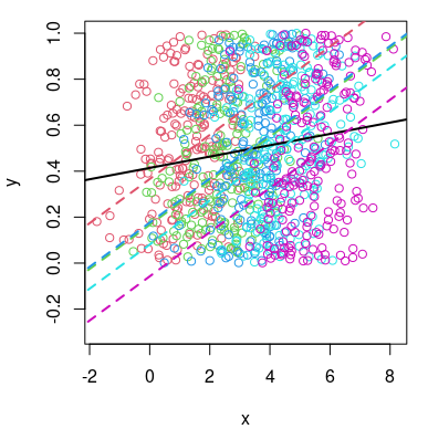
Below is an example of the situation.

• black line: fit with without mixed effect.
• coloured lines: fits with mixed effects, each colour is for a different group.

Instead of fitting one line through all points which will be more or less flat, you get to fit lines through the coloured points instead.

It is very similar to the change of fixed effects when adding an additional regressor (the difference is only that a random effect has a restriction in being considered normal distributed and adds a term to the likelihood).

Here is a related question about the coefficient change with an answer containing links to many related questions Why do my (coefficients, standard errors & CIs, p-values & significance) change when I add a term to my regression model?

---

Random effects sum to zero

Why do the random effects sum to zero or not? The answer below is not a rigorous proof, but it will provide an intuition behind it. I am writing it down a bit as bullet points because when I try to describe it in detail then I get a stuck in my words.

I am using an example computation that manually computes the random effects model. It gives the same results as the glmerfunction.

Example computation

I am making an adaptation of your example

• With two groups instead of five groups. In this way it is easier to make plots later on.
• For the second group I am changing the level to generate the y_bin values (0.1 instead of 0.5). This will make the effect of the random effects not summing up to zero larger. (and this makes it less ambiguous whether this effect is due to a computation error or not)

Plots of this data look like this

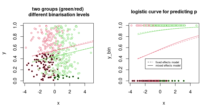
In these plots I have fitted both a fixed and a mixed effects model. What you can notice here is that the fitted lines for the two groups are closer together with the mixed effects model. This is an effect of regarding the effect as a random effect. By assuming that the effect follows a normal distribution you will get some shrinking of the effects because the model prefers the effects to be closer to zero (where the probability is higher).

The likelihood function is an integral

The random effects that you obtain with ranef(mod_logistic)$group are not coefficients/parameters of the model. They are nuisance parameters which glmer integrates out of the likelihood function. What the model returns are point estimates but in reality they follow a distribution.

The likelihood function considering all parameters (intercept, $\alpha$, slope $\beta$, standard deviation for random effects distribution $\sigma$) given the data (binary outcome $y$, regressor $x$, $\text{group}$ and random effects $z_1, z_2$) is

$$\mathcal{L}(\hat\alpha,\hat\beta,\hat\sigma | z_1, z_2,x,y,\text{group}) = \prod_{i=1}^n \hat{p}_i^y(1-\hat{p}_i)^{1-y} \cdot \prod_{i=1}^2 \frac{1}{\hat\sigma \sqrt{2\pi}} \exp \left(-\frac{z_i^2}{2 \hat\sigma} \right) \\ \text{where $\hat{p}_i = \hat\alpha + \hat\beta \cdot x + z_1 \cdot \mathbb{I}_{\text{group = 1}} + z_2 \cdot \mathbb{I}_{\text{group = 2}}$} $$

But we do not observe the random effects $z_i$ directly nor do we consider them as parameters and they are integrated out to obtain a marginal likelihood

$$\begin{array}{} \mathcal{L}(\hat\alpha,\hat\beta,\hat\sigma|x,y,\text{group}) &=& \iint_{z_1,z_2 \in \mathbb{R}^2} \mathcal{L}(\hat\alpha,\hat\beta,\hat\sigma | z_1, z_2,x,y,\text{group}) \, \text{d} z_1 \, \text{d} z_2 \\ &=& \iint_{z_1,z_2 \in \mathbb{R}^2} \prod_{i=1}^n \hat{p}_i^y(1-\hat{p}_i)^{1-y} \cdot \prod_{i=1}^2 \frac{1}{\hat\sigma \sqrt{2\pi}} \exp \left(-\frac{z_i^2}{2 \hat\sigma} \right) \, \text{d} z_1 \, \text{d} z_2 \end{array} \\ \text{where $\hat{p}_i = \hat\alpha + \hat\beta \cdot x + z_1 \cdot \mathbb{I}_{\text{group = 1}} + z_2 \cdot \mathbb{I}_{\text{group = 2}}$} $$

Plots of the likelihood

In the plot below we keep the parameters alpha, beta and sigma fixed at the level of the optimum obtained by glmer and see how the first likelihood function changes as function of the two random effects.

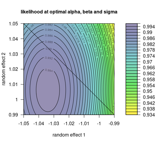
The difference from the line where the effects are exactly opposite is large. The difference is not due to a computational error. The maximum likelihood is truly in the point around -1.034, 1.006.

It is this point which glmer returns with the function ranef(mod_logistic)$group (or actually I am not sure, maybe they use the weighted average but in both cases you get more or less the same value).

We can increase the likelihood function by changing the value of the fixed intercept (alpha) with $\frac{-1.033890 + 1.006397}{2}$, then instead of a maximum at $-1.033890, 1.006397$ we get a maximum at $-1.020144, 1.020144$.

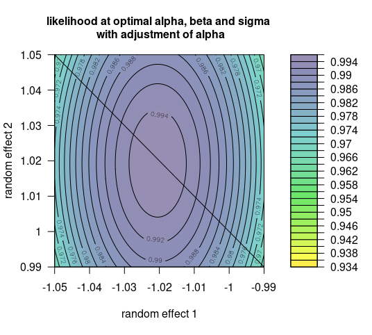
However, while we have for this new point a higher maximum in terms of the first likelihood function, the likelihood has decreased in terms of the second likelihood function. The reason is because the second likelihood function is not only about the maximum for a particular point of random effects $-1.020144, 1.020144$, instead it integrates over the entire space.

By changing the intercept we can make the peak of the likelihood function higher but not the integral.

What is going on

The following viewpoint might help to gain some intuition.

For the case of two groups we could re-parameterize the random effects in terms of the independently normal distributed variables $u = 0.5(z_1 + z_2)$ and $v = 0.5(z_1 - z_2)$. Then, using the group variable having either values $-1$ or $1$, the likelihood functions become:

$$\mathcal{L}(\hat\alpha,\hat\beta,\hat\sigma | u,v,x,y,\text{group}) = \prod_{i=1}^n \overbrace{\hat{p}_i^y(1-\hat{p}_i)^{1-y}}^{\text{probability of $y_{bin}$ outcome}} \cdot \overbrace{ \frac{1}{\hat\sigma \sqrt{2\pi}} \exp \left(-\frac{u^2+v^2}{2 \hat\sigma} \right) }^{\text{probabiltiy of random effects}} \\ \text{where $\hat{p}_i = \hat\alpha + \hat\beta \cdot x + u + v \cdot \text{group}$} $$

$$\mathcal{L}(\hat\alpha,\hat\beta,\hat\sigma|x,y,\text{group}) = \iint_{u,v \in \mathbb{R}^2} \prod_{i=1}^n \hat{p}_i^y(1-\hat{p}_i)^{1-y} \cdot \frac{1}{\hat\sigma \sqrt{2\pi}} \exp \left(-\frac{u^2 + v^2}{2 \hat\sigma} \right) \, \text{d} u \, \text{d} v \\ \text{where $\hat{p}_i = \hat\alpha + \hat\beta \cdot x + u + v \cdot \text{group}$} $$

We have that $\mathcal{L}(\hat\alpha,\hat\beta,\hat\sigma | u,v,x,y,\text{group})$ is maximized when $u = 0$, but the parameters $\hat\alpha,\hat\beta,\hat\sigma$ for which this is optimized may not need to be the same parameters for which $\mathcal{L}(\hat\alpha,\hat\beta,\hat\sigma|x,y,\text{group})$ is optimized.

There is a certain interaction between $\hat\beta$ and $u$. In the prediction of $\hat{p_i} = \hat\alpha + \hat\beta \cdot x + u + v$ we have that we can change $\hat\beta$ and $u$ while keeping the sum the same. Then the first part of the likelihood function, the probability of the $y_{bin}$ outcomes, remains unchanged, but the second part, the probability of the random effects changes. So for whatever set of values $\alpha,\beta,\sigma,u,v$, if we have $u \neq 0$, then $\mathcal{L}(\hat\alpha+u,\hat\beta,\hat\sigma | 0,v,x,y,\text{group})> \mathcal{L}(\hat\alpha,\hat\beta,\hat\sigma | u,v,x,y,\text{group})$

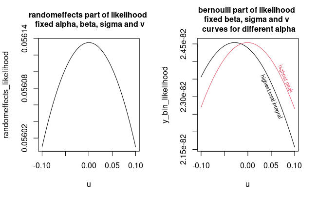
In the image below we plot these parts of the likelihood function seperately in the left and the right pane

$$\begin{array}{rcl} \text{Bernoulli part} &:& \prod_{i=1}^n \hat{p}_i^y(1-\hat{p}_i)^{1-y} \\ \text{random effects part} &:& \frac{1}{\hat\sigma \sqrt{2\pi}} \exp \left(-\frac{u^2 + v^2}{2 \hat\sigma} \right) \end{array}$$

We get the highest peak in the likelihood fucntion by choosing a $\alpha$ such that the two parts align. In this case the peak will occur in $u=0$ and the sum of the random effects will be zero.

However, the curve on the right pane, the Bernoulli part of the likelihood function, is not entirely symmetric and we get that the optimum for the integral (in which case, btw. we also vary $v$) will occur with an alpha for which the peak of the product will not occur in $u=0$.

In linear regression instead of glm you have that the function is not a Bernoulli distribution, but instead a Gaussian distribution. In that case the optimum for the integral will occur when we also have the peak at $u=0$.

Code

library(lmerTest)
library(pracma)
layout(matrix(1:2,1))

############### fake data
set.seed(1)
n = 200

group <- rep(1:2, each = n)
y <- runif(2*n)
y_bin <- (y > .9 - .4*group)
x <- 0.5*y + rnorm(n*2) + group*2
x <- x-mean(x)

############ plot y
plot(x,y, col = 1+group, ylim = c(0,1), cex = 0.7, pch = 21, bg = c(1,0)[y_bin+1],
     main = "two groups (green/red) \n different binarisation levels", cex.main = 1)

### add fitted lines linear model for y
mod0 <-  lm(y ~ x + group)
mod <- lmer(y ~ x + (1|group))
u = seq(-3,25,0.1)

lines(u,mod0$coefficients[1] + mod0$coefficients[2]*u + mod0$coefficients[3],   col = 2, lwd = 1, lty  = 2)
lines(u,mod0$coefficients[1] + mod0$coefficients[2]*u + mod0$coefficients[3]*2, col = 3, lwd = 1, lty  = 2)
lines(u,mod@beta[1] + ranef(mod)$group[1,1] + (mod@beta[2])*u, col = 2, lwd = 1, lty  = 1)
lines(u,mod@beta[1] + ranef(mod)$group[2,1] + (mod@beta[2])*u, col = 3, lwd = 1, lty  = 1)


########### plot y_bin
plot(x,y_bin, col = 1+group, ylim = c(0,1), cex = 0.7, pch = 21, bg = c(1,0)[y_bin+1],
     main = "logistic curve for predicting p", cex.main = 1)

### add fitted lines for logistic regression
mod_logistic0 <-  glm(y_bin ~ x + group, family="binomial")
mod_logistic <- glmer(y_bin ~ x + (1|group), family="binomial", 
                      control = glmerControl(boundary.tol = 10^-7,  tolPwrss = 10^-10), nAGQ = 100, verbose = 2)
u = seq(-3,25,0.1)
lines(u, (exp(-mod_logistic0$coefficients[1] - mod_logistic0$coefficients[2]*u - mod_logistic0$coefficients[3])+1)^-1 , col  = 2, lwd = 1, lty = 2)
lines(u, (exp(-mod_logistic0$coefficients[1] - mod_logistic0$coefficients[2]*u - mod_logistic0$coefficients[3]*2)+1)^-1 , col  = 3, lwd = 1, lty = 2)
lines(u, (exp(-mod_logistic@beta[1] - mod_logistic@beta[2]*u - ranef(mod_logistic)$group[1,1])+1)^-1 , col = 2, lwd = 1)
lines(u, (exp(-mod_logistic@beta[1] - mod_logistic@beta[2]*u - ranef(mod_logistic)$group[2,1])+1)^-1 , col = 3, lwd = 1)

legend(-2,0.4, c("fixed effects model", "mixed effects model"), cex = 0.6, lty = c(2,1))

### sum of random effects is -0.02749356
sum(ranef(mod_logistic)$group)


############ Likelihood functions

logLikelihood = function(par) {
  alpha = par[1]
  beta = par[2]
  sigma = par[3]
  re = par[c(4,5)]
  p = (exp(-alpha - beta * x - re[group])+1)^-1
  ll = sum(log(p)*y_bin) + sum(log(1-p)*(1-y_bin)) - 2*0.5 * log(2*pi) - 2*log(sigma) - 0.5/sigma^2 * sum(re^2)
  return(-ll)
}

### function to compute likelihood similar to logLikelihood
### we use an additional constant 'logscale' to prevent very small or larger values
Likelihood = function(re1, re2, par3, logscale = 190.79) {
  re = c(re1,re2)
  alpha = par3[1]
  beta = par3[2]
  sigma = abs(par3[3])
  p = (exp(-alpha - beta * x - re[group])+1)^-1
  ll = sum(log(p)*y_bin) + sum(log(1-p)*(1-y_bin)) - 2*0.5 * log(2*pi) - 2*log(sigma) - 0.5/sigma^2 * sum(re^2) + logscale
  return(exp(ll))
}

### Likelihood function that integrates over nuisance parameters
logLikelihood_int = function(par) {
  d = 5
  int = pracma::integral2(Likelihood, center[1]-d,center[1]+d,center[2]-d,center[2]+d,  par3=par, vectorized = 0)
  return(-log(int$Q))
}


############ Solving the optimization problems

### optimize likelihood including nuisance parameters in optimization
opt1 = optim(par = c(0,0,1,0,0), fn = logLikelihood, lower = c(-Inf,-Inf,0.01,-Inf,-Inf), method = "L-BFGS-B", 
      control = list(trace = 1, factr = 4) )
opt1

### use the estimate from the first model to define the center of the area for integration
center = opt1$par[4:5]

### optimize likelihood integrating over nuisance parameters in optimization
opt2 = optim(par = opt1$par[1:3], fn = logLikelihood_int, method = "Nelder-Mead", 
             control = list(trace = 1) )
opt2


### Compare results      alpha      beta       sigma      r1         r2
ranef(mod_logistic) #                                     -1.033890  1.006397
mod_logistic@beta   #    1.3165318  0.2361008  
mod_logistic@theta  #                          1.055184
opt1$par            #    1.3004738  0.2363676  1.0164584  -1.0164576 1.0164576
opt2$par            #    1.3167908  0.2362038  1.0550018



layout(matrix(1,1))


cplot = function(middle = c(-1.02,1.02), size = 150, d = 0.0002, 
                 adjustment= c(0,0,0),
                 axislevs1 = seq(-1.07,-0.98,0.01), axislevs2 = seq(0.97,1.05,0.01),
                 levels = seq(0.934,0.996,0.002), title = "") {
  ### choose variable range
  e1 <- middle[1] + d*c(-size:size)
  e2 <- middle[2] + d*c(-size:size)
  n <- length(e1)

  ### compute results on a matrix
  z <- matrix(rep(0,n*n),n)
  
  for (i1 in 1:n) {
    for (i2 in 1:n) {
      z[i1,i2] = Likelihood(e1[i1],e2[i2], opt2$par + c(adjustment,0,0) )
    }
  }

  ### getting coordinates of maximum
  m = which.max(z)
  m1 = m %% n
  m2 = ceiling(m/n) 
  max = max(z)
  max_coordinate = c(e1[m1], e2[m2])
  
  range(z)
  
  #plotting parameters
  levs <-    levels   # contour levels
  collevs <- levels   # colour levels

  #labs <- (matrix(levs[-c(1)],1/0.5))  # for contour labels
  #labs[-1/0.5,] <- ""
  #labs <- c("",as.character(labs))
  labs = levs
  
  # contour plot
  filled.contour(e1,e2,(z),
                 xlab="random effect 1", ylab="random effect 2", border = NULL,       
                 color.palette=function(n) {hsv(c(seq(0.15,0.7,length.out=n),0),
                                                c(seq(0.7,0.2,length.out=n),0),
                                                c(seq(1,0.7,length.out=n),0.9))},
                 levels=collevs,  
                 key.axes=axis(4,at=levs,labels=labs),
                 plot.axes= c({
                   contour(e1,e2,(z),add=1, levels=levs, 
                           labels= labs, vfont = c("sans serif", "plain"))
                   axis(1, at = axislevs1,labels=axislevs1)
                   axis(2, at = axislevs2,labels=axislevs2)
                   lines(c(-2,2),c(2,-2))
                   #points(max_coordinate[1] , max_coordinate[2], pch = 21, col = 1, bg = 2, cex = 0.7)
                   title(title, cex.main = 1)
                 },"")
  )
  return(max(z))
}

cplot(title = "likelihood at optimal alpha, beta and sigma")
cplot(adjustment = c(sum(ranef(mod_logistic)$group)/2,0,0),
      title = "likelihood at optimal alpha, beta and sigma \n with adjustment of alpha")


layout(matrix(1:2,1))

par = as.numeric(c(mod_logistic@beta,
        mod_logistic@theta,
        ranef(mod_logistic)$group[,1]))

Likelihood_parts = function(par) {
  alpha = par[1]
  beta = par[2]
  sigma = abs(par[3])
  re = par[4:5]
  p = (exp(-alpha - beta * x - re[group])+1)^-1
  ll1 = sum(log(p)*y_bin) + sum(log(1-p)*(1-y_bin)) 
  ll2 =  - 2*0.5 * log(2*pi) - 2*log(sigma) - 0.5/sigma^2 * sum(re^2)
  return(c(exp(ll1),exp(ll2)))
}

u = seq(-0.1,0.1,0.001)
randomeffects_likelihood = sapply(u, function(x) Likelihood_parts(par+(-sum(par[4:5])/2 + x/2)*c(0,0,0,1,1))[2])
plot(u,randomeffects_likelihood, type = "l")
title("randomeffects part of likelihood \n fixed alpha, beta, sigma and v", cex.main = 1)


y_bin_likelihood = sapply(u, function(x) Likelihood_parts(par+(-sum(par[4:5])/2 + x/2)*c(0,0,0,1,1))[1])
plot(u,y_bin_likelihood, type = "l")
title("bernoulli part of likelihood \n fixed beta, sigma and v  \n curves for different alpha", cex.main = 1)

f#or (i in 1:5) {
#  parc = c(1.317-i*0.01,par[2:5])
#  y_bin_likelihood = sapply(u, function(x) Likelihood_parts(parc+(-sum(par[4:5])/2 + x/2)*c(0,0,0,1,1))[1])
#  lines(u,y_bin_likelihood, col = 4, lty = 2)
#}

y_bin_likelihood = sapply(u, function(x) Likelihood_parts(par+(-sum(par[4:5])/2 + x/2)*c(0,0,0,1,1) + c(sum(par[4:5])/2,0,0,0,0))[1])
lines(u,y_bin_likelihood, col = 2) 

text(0.05, 2.3*10^-82, "highest total integral", cex = 0.7, srt = -67)
text(0.08, 2.35*10^-82, "highest peak", cex = 0.7, srt = -67, col = 2)