I would like to complement @kqr's answer.
We don't plug in the (unknown) true proportion in the formula for the confidence interval, we plug in the sample proportion $\hat{p}$: it's $\hat{p} + z_{1-\alpha}\sqrt{\hat{p}(1-\hat{p})/n}$ instead of $p + z_\alpha\sqrt{p(1-p)/n}$. The sample sizes quoted by @kqr don't account for sampling variability. Of course it's hard to account for it because we only know $\hat{p}$ after we collect the data. So what can we do?
One option is power analysis as suggested by @whuber. An alternative is to plan for the desired precision of the estimate as suggested by @kqr.
I think it's more useful to plan for precision. This means to calculate the sample size to achieve a specific margin of error $\delta$. Usually the margin of error is defined as the half-length of a two-sided confidence interval. But you are interested in testing a one-sided hypothesis, so let's define the margin of error as the upper half of a one-sided confidence interval, just as @kqr does. This amounts to using $z_{1-\alpha}$ instead of $z_{1-\alpha/2}$ as the critical value.
$$
\begin{aligned}
\delta = z_{1-\alpha}\operatorname{SE}/\sqrt{n}
&& \Leftrightarrow &&
n = \left(\frac{z_{1-\alpha}\operatorname{SE}}{\delta}\right)^2
\end{aligned}
$$
The formula for the required sample size $n$ has three ingredients: The critical value $z_{1-\alpha}$ is a function of the significance level $\alpha$. For a sample proportion, the standard error $\operatorname{SE}$ is given by $\sqrt{\hat{p}(1-\hat{p})}$. And the margin of error $\delta$ depends on the accuracy you want to achieve; for example, you may decide you want to estimate the error rate with a 0.5% accuracy. As I already mentioned, specifying $\operatorname{SE}$ is a bit tricky. If you believe the true error rate is between 0.8% and 1.2% it's better to plug in 1.2% than 1%; this will give a slightly more conservative $\operatorname{SE}$ = 0.325 (instead of $\operatorname{SE}$ = 0.3).
alpha <- 0.05
p_se <- .012
delta <- .005

(qnorm(1 - alpha) * sqrt(p_se * (1 - p_se)) / delta)^2
#> [1] 1283.077
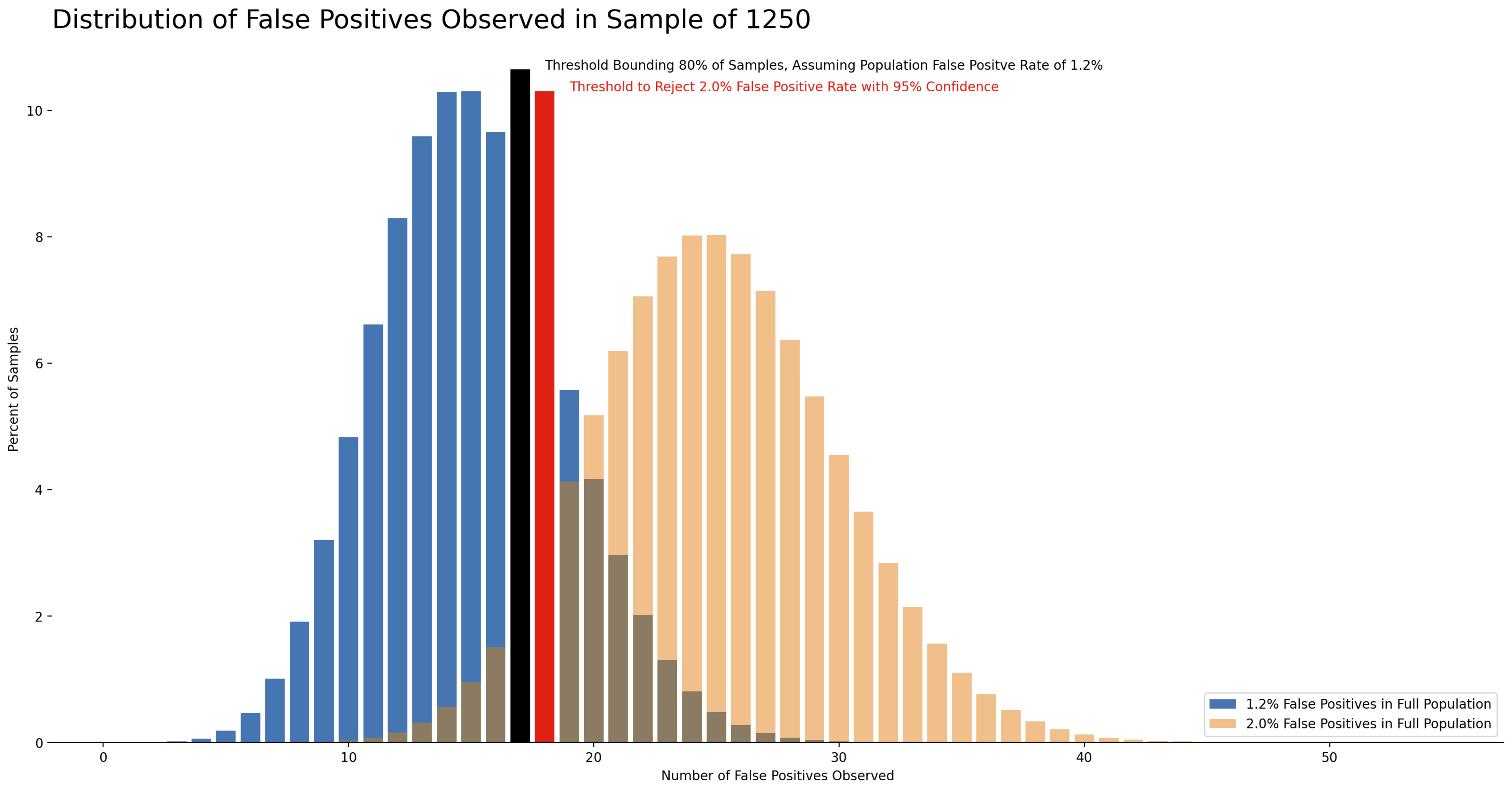
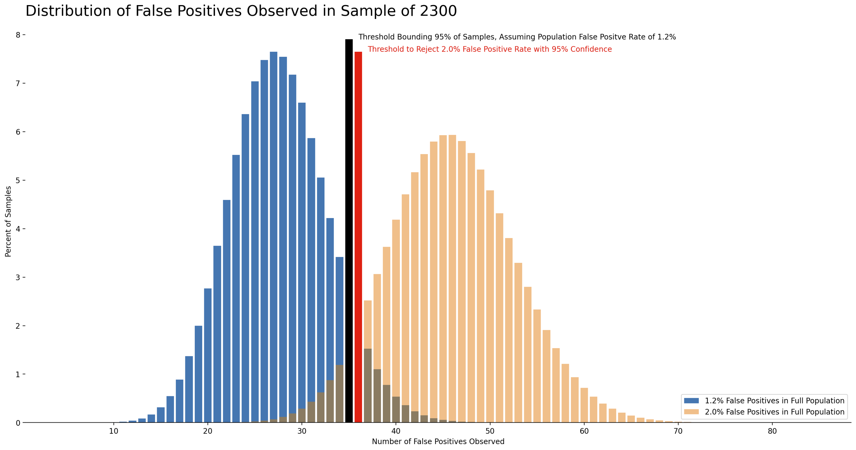
Power analysis also has three ingredients: the probability $\alpha$ of type I error (aka significance level), the probability $\beta$ of type II terror (power = 1 - $\beta$) and the effect size (it's a function of the difference between the true error rate and the 2% error rate you want to detect). In your question you don't commit to specific values for the a-priori error rate and the power. However, you would have to put down those numbers to make sample size calculations. There is no other way to get a "guarantee" in statistics.
Here's how to do it in R. The null hypothesis is $H_0$: p = 0.02, the alternative hypothesis is $H_1$: p = 0.01. Let's calculate the sample size for a less-than z-test for a proportion with $\alpha$ = 0.05 and power = 0.90. That is, there is 5% probability that the null is incorrectly rejected when it is true, and 10% probability that the null is not rejected when it is not true.
library("pwr")

alpha <- 0.05
power <- 0.9

p <- 0.01
q <- 0.02

pwr.p.test(h = ES.h(p, q), sig.level = alpha, power = power, alternative = "less")$n
#> [1] 1229.475
The two analyses agree that the required sample size is at least 1,200. Both "recipes" have three ingredients; the common ingredient is the significance level $\alpha$. The distinction is in what you control for in the computation: the precision of the estimate or the power of the significance test.


