Calculate the likely number of distinct categorical values (diagnoses) for a patient population

Question

In healthcare, patient diagnosis is recorded with a code called an ICD code. There are around 43K distinct diagnosis codes. So, basically any population can have between 0 and 43K DISTINCT diagnosis. To keep things simple, assuming that:

1. Every diagnosis is equally likely
2. Each patient has just 1 diagnosis

... how do I estimate the number of distinct diagnoses in a patient population of N?

Answer 1

This is related to the Coupon collector's problem as noted in the comments.

Building off of this post, the probability of observing $k$ unique letters in $m$ random uniform samples from an alphabet of size $n$ is:

$$\bigg\{\!{m\!\atop{k}}\bigg\}\binom{n}{k}\frac{k!}{n^m}=\bigg\{\!{m\!\atop{k}}\bigg\}\frac{n!}{n^m(n-k)!}$$

Where $\big\{\!{m\!\atop{k}}\big\}$ is the Stirling number of the second kind.

For large $m$, $\big\{\!{m\!\atop{k}}\big\}$ can be approximated (original paper):

$$\left\{{m \atop k}\right\} \sim \sqrt{\frac{v-1}{v(1-G)}} \left(\frac{v-1}{v-G}\right)^{m-k} \frac{k^m}{m^k} e^{k(1-G)}\binom{m}{k}$$

where $v=m/k$, and $G\in(0,1)$ is the unique solution to $G=ve^{G-v}$.

Here is an R function that returns the probability of every $k$:

library(copula)

coupons1 <- function(n, m) {
  l <- min(m, n)
  k <- 1:l
  if (m < 200) {
    logS <- log(Stirling2.all(m)[k])
  } else {
    # estimate the log Stirling numbers
    v <- m/k
    G <- 1/v
    vexpv <- v/exp(v)
    # five Newton-Raphson iterations to solve for `G`
    # (could be modified to check convergence at each iteration)
    for (i in 1:5) G <- G - (G - (vexpG <- vexpv*exp(G)))/(1 - vexpG) 
    logS <- (log(v - 1) - log(v*(1 - G)))/2 + lchoose(m, k) +
      (m - k)*(log(v - 1) - log(v - G)) + m*log(k) - k*log(m) + 
      k*(1 - G)
    if (l == m) logS[m] <- 0
  }
  pmf <- exp(logS + lgamma(n + 1) - lgamma(n - k + 1) - m*log(n))
  pmf/sum(pmf)
}

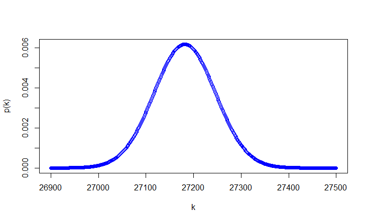
The probability of $k=1,2, \dotsc, 43000$ for $n=m=43000$:

system.time(k1 <- coupons1(43e3, 43e3))
#>    user  system elapsed 
#>    0.02    0.00    0.01

plot(26900:27500, k1[26900:27500], xlab = "k", ylab = "p(k)", col = "blue")

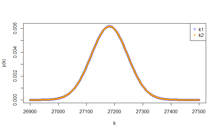
Comparing that result to a brute-force approach:

Rcpp::cppFunction("
  NumericVector coupons2(const int& n, const int& m) {
    int maxk;
    int n1 = n - 1;
    if (n > m) {
      maxk = m;
    } else {
      maxk = n;
    }
    
    NumericVector k (maxk);
    k(0) = 1;
    
    for (int i = 1; i < maxk; i++) {
      for (int j = i; j > 0; j--) {
        k(j) = (k(j - 1)*(n - j) + k(j)*(j + 1))/n;
      }
      k(0) = k(0)/n;
    }
    
    for (int i = maxk; i < m; i++) {
      for (int j = n1; j > 0; j--) {
        k(j) = (k(j - 1)*(n - j) + k(j)*(j + 1))/n;
      }
      k(0) = k(0)/n;
    }
    
    return k;
  }
")

system.time(k2 <- coupons2(43e3, 43e3))
#>    user  system elapsed 
#>   12.29    0.00   12.31

The relative error from using the Stirling number approximation is small for a large $m$.

max(abs(k1[26900:27500] - k2[26900:27500])/k2[26900:27500])
#> [1] 8.288009e-07

points(26900:27500, k2[26900:27500], col = "orange", pch = 20)
legend("topright", legend = c("k1", "k2"), col = c("blue", "orange"), 
        pch = c(1, 20))

---

A note on the occupancy R package

The occupancy package features the distribution for this problem, with an option for exact or approximate calculations. docc returns the PMF of k. However, it is much slower than coupons1 and coupons2 above, with the computation time growing approximately geometrically for $m=n$. Additionally, the approximation provided is poor compared to the one provided by coupons1:

n <- 43e3L
system.time(k3 <- occupancy::docc(1:n, n, n, approx = TRUE))
#>    user  system elapsed 
#>    1.61    2.00    3.61
max(abs(k3[26900:27500] - k2[26900:27500])/k2[26900:27500])
#> [1] 0.01156602

Time occupancy::docc for $m=n=4300$ with approx = FALSE:

n <- 4300L
system.time(occupancy::docc(1:n, n, n))
#>    user  system elapsed 
#>   35.58    0.14   35.75