Predicted Probability of GAMM
I've probably beaten this topic to death here, but I continue to have issues with model fitting. Thanks to the excellent advice here, I was able to at least square away what was programmed correctly. However I have run into two new problems. First, fitting a gamm4 object is extremely time-consuming (already warned about in the last post), as I left R running last night and it was still trying to fit my model this morning. Instead I used the advice to fit using bam as suggested with this code:
fit <- bam(Outcome
    ~ s(Control_1) # control vars
    + s(Control_2)
    + s(X1) # main effects
    + s(X2)
    + s(X3)
    + s(Main) # main variable of interest
    + ti(Main, X1, k = c(5, 5)) # tensor interactions
    + ti(Main, X2, k=c(5,5))
    + ti(Main, X3, k=c(5,5)),
    + s(Subject.ID, bs = "re")
    + s(Item.ID, bs = "re"), # random effects
    data= data,
    family=binomial) # logistic
I have two models with this code...the only difference is the outcome variable. One model fits fairly quickly because it has far fewer items and thus fewer observations. The other, which is more than 50k observations, is usually extremely time consuming and thus bam is helpful for fitting it faster.
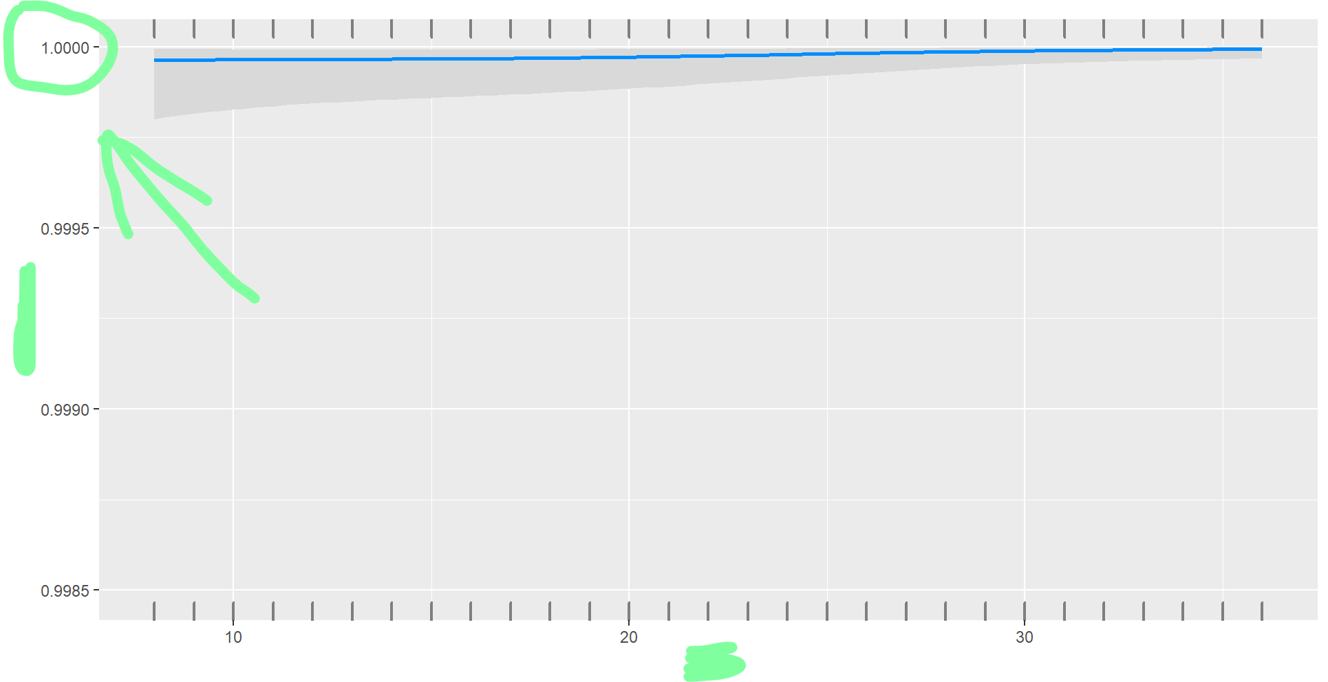
My second problem, however, is that my GAMM fit for this larger model seems to be giving me impossible predicted probability compared to the GLMM model I previously used. Most of the predictors look like this when I plot them with visreg:
visreg(fit,
       "Control",
       scale = "response",
       gg=T)
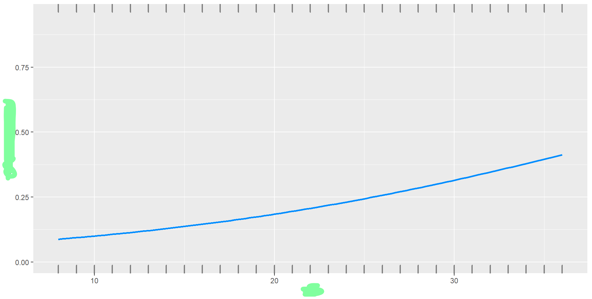
You can see here that almost everyone is scoring 1 on the outcome. But that is simply not possible given the actual raw probability of scores, which calculated like so gives me 42.3%:
21715/sum(21715+29585)
Plotting by Linear Argument
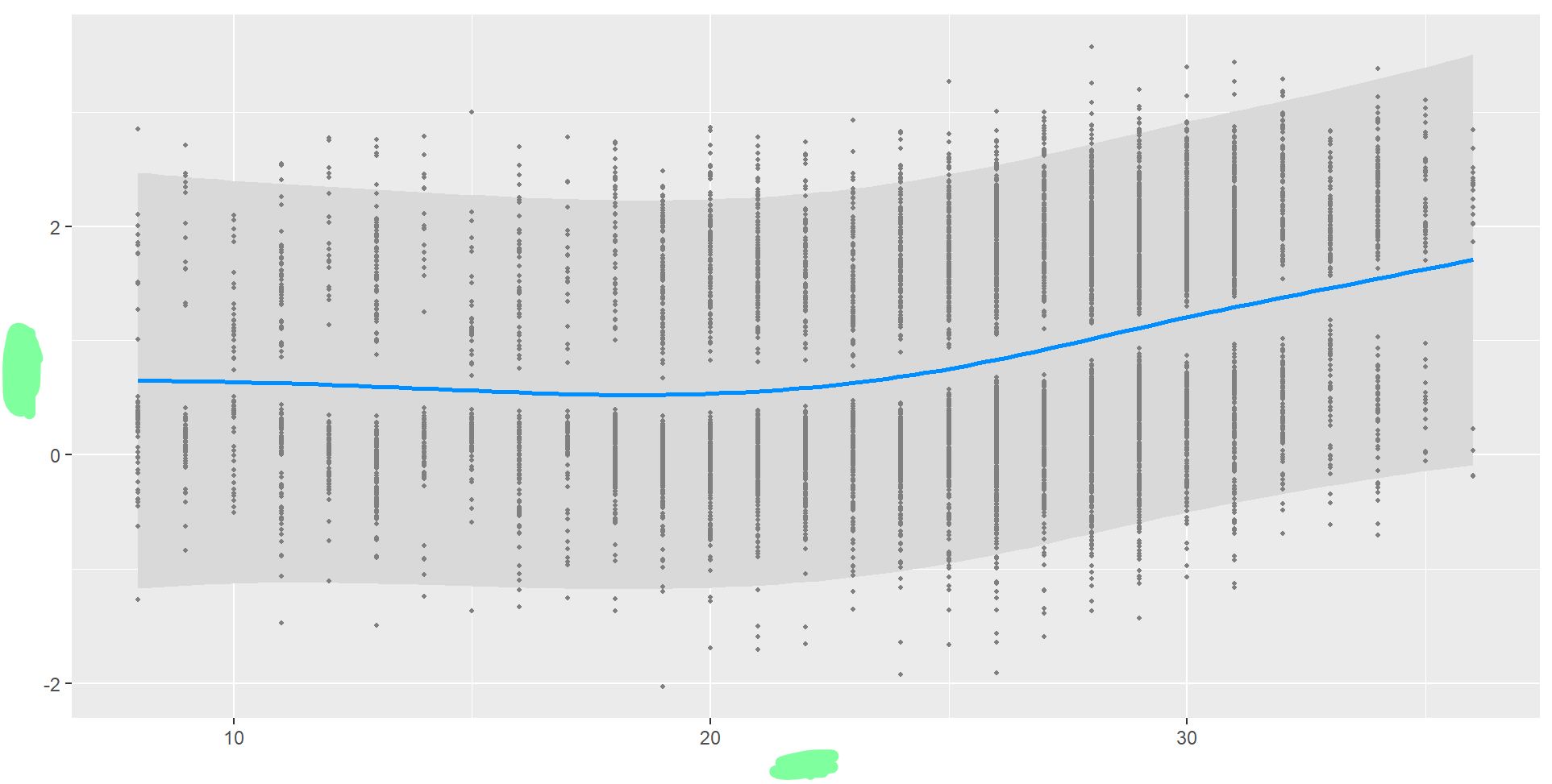
When plotting the same predictor via the linear argument, it looks more normal:
GLMM Comparison
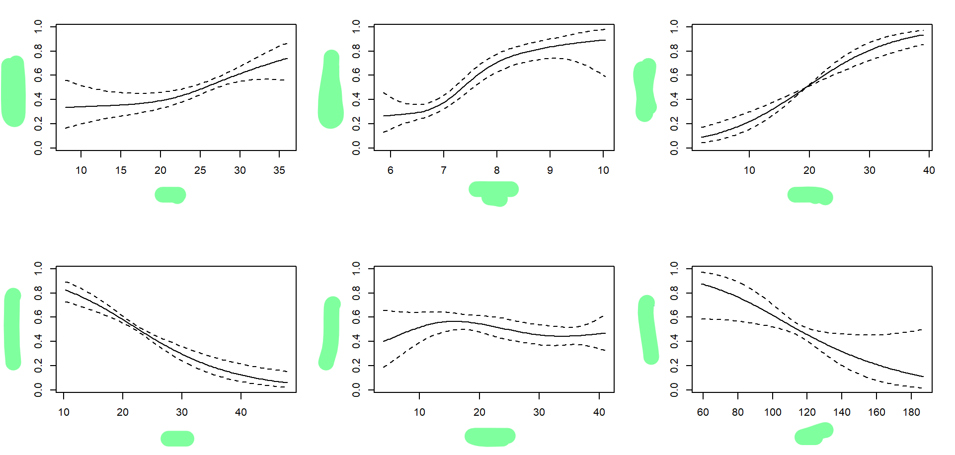
For the previous GLMM version of this model, the coefficients were fairly similar. That said, the predicted probability is completely different:
Here it seems the predicted probability is much more likely and the relationship makes sense.
Am I simply missing something by plotting the predicted probability this way? Is scaling the predictor by response not normal in GAMMs? It seems all else considered, the DHARMa residuals perform very well and the coefficients match up mostly to the expected coefficients of the GLMM. The large model also explains about 66% of the deviance whereas the smaller model only explains about 33.3%, so it doesn't appear to be overfitting as far as I can tell.


