Reason why kernel density graphs are so different in Python versus R

Question

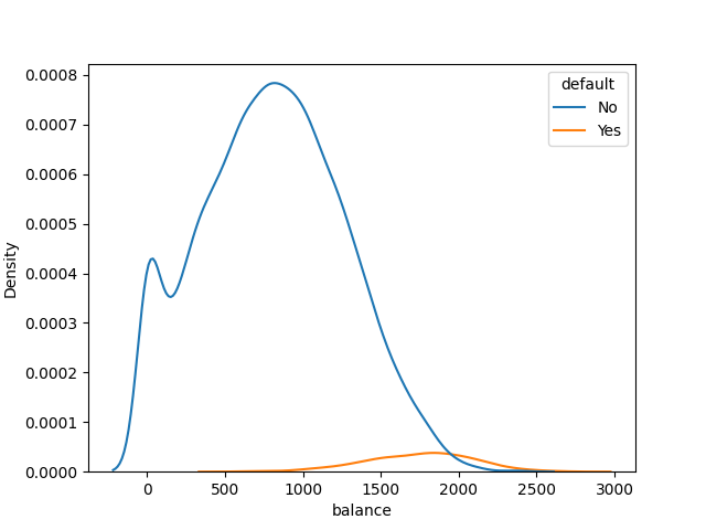
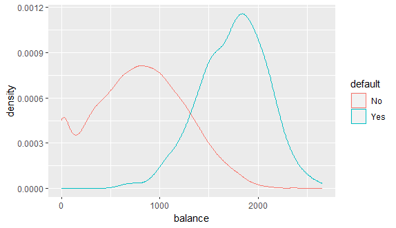
I plotted the same data in R using geom_density, but the blip for "Yes" is much, much smaller in Python using kdeplot from Seaborn than for R.

I am using the dataset default from the ISLR package. It's included for R and I downloaded it for Python from this link.

R code:

install.packages("ISLR")
install.packages("tibble")
install.packages("ggplot2")

library("ISLR")
library("tibble")
library("ggplot2")
df <- as_tibble(Default)

p <- ggplot(df, aes(x=balance, color=default)) + 
  geom_density()

Output:

Python code:

import seaborn as sns
import matplotlib.pyplot as plt
import pandas as pd

default = pd.read_excel(r"")

sns.kdeplot(data=default, hue='default', x="balance")
plt.show()

Output:

I'm following this tutorial on logistic regression.

Can anyone explain to me in detail how the implementation in kdeplot versus geom_density results in these different graphs? I read the docs (kdeplot, geom_density) but I'm can't see a clear reason.

I really want to understand as I use Python for my work as a data analyst, want to learn forecasting techniques for my job, and would like to also learn R. I don't have much statistics background but I have calculus background, if that's relevant to understanding the differences.

Answer 1

In the R version, the two curves are kernel density estimates for the densities in the two groups. The area under each curve is 1.

According to the documentation you linked, kdeplot has an option

common_norm bool If True, scale each conditional density by the number of observations such that the total area under all densities sums to 1. Otherwise, normalize each density independently.

The default is True, so that's what you got. This means that the two curves are rescaled density estimates in the two groups. Rather than the area under each curve being 1, as it is for a density, the area has been scaled to be proportional to the number of observations in the group. The numbers are

> table(Default$default)

  No  Yes 
9667  333 

So in the Python version the Yes curve is scaled to about 3.4% of the height of the No curve, but you can fix this with the common_norm option.