Incorporating a random effect to the null model

Question

I would like to decide if it is reasonable to include a factor variable to the null model I.e y ~ 1 VS y ~ (1|x)

I haver read this answer https://stats.stackexchange.com/a/56157/21521 which suggest obtaining the p-value or AIC values from anova(y ~ 1, y ~ (1|x)) but I have my doubts. First of all lme4 does not allow to fit the null model so I have to perform anova with different type of objects (Is this ok?)

anova( lmer(y ~ (1| x) , REML = FALSE), lm(y ~ 1))

Now the issues I find is that anova considers only one extra parameter for the factor variable which has many levels. This makes me suspicious of AIC and BIC. Also a short simulation under the null model shows the test is over conservative since p-values are not uniformly distributed and concentrate around one.

library(lme4)
set.seed(1)
x = rep(c('a','b','c'), 100)

simulate_pvalue = function(){
                     y = rnorm(length(x)) 
                     fit1 = invisible(lmer(y ~ (1| x) , REML = FALSE))
                     fit0 = lm(y ~ 1)
                     anova(fit1, fit0)$`Pr(>Chisq)`[2]
}
p_values = replicate(1000, simulate_pvalue() )
hist(p_values)

• Is it ok to perform anova with an lm and and lme4 objects?
• Is there anything better I could be doing?

Answer 1

I will try to address why in many cases, integrating or not a random effect is a design question not a statistical one. Also, I will provide conceptual ideas on why anova test on linear mixed model is a overconservative procedure. All the code used for the post is given at the end.

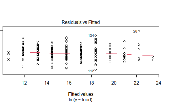
Let's start with a brief example. Let's say you have a set of 100 mice, for each mouse you have 3 repeated measures of their food consumption and activity. We can expect correlation for mouse food and activity. You want to test whether the mouse activity is associated with food consumption. Simulating some random data and fitting a linear regression we see that something is going wrong when we plot the residuals against fitted values.

Indeed, the plot does not show random distribution, but patterns can be clearly observed. It suggests that we have some hierarchy in your data (of course we have since we simulated a random intercept).

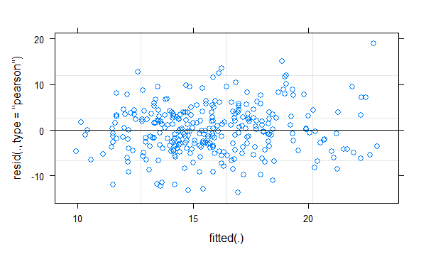
Now we fit a linear mixed regression model, including a random intercept for mouse. Now it is what we see:

We now respect our model assumption. However, testing whether we need to include a random intercept, we see that we cannot accept H1 (variance>=0). If you do so, you will obtain trouble with your residual plot.

Additionally: In your Anova table, you have 3 parameters for your linear model (1 intercept, 1 slope and 1 population variance) while in the linear mixed model 4 parameters (1 intercept, 1 slope, 1 population variance and 1 random-effect variance). Nothing differs much except your validation plots.

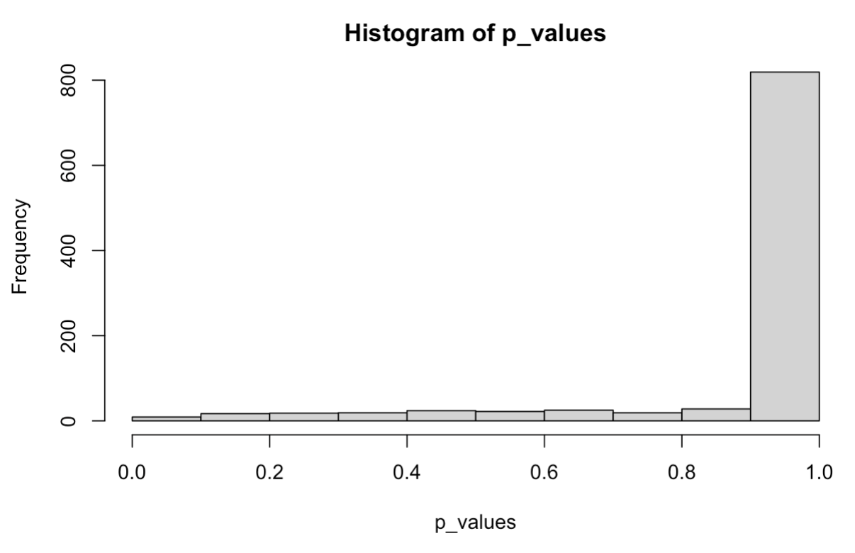
Finally, just an extra section for the overconservative behavior. This behavior is mainly due to the unknown asymptotic distribution for the test statistic. Using bootstrap procedure may be a good option. Technically speaking, is because our test is on boundary condition (>=0).

I hope I clarify why random effect is often a design question. Statistics alone are rarely enough.

Hope this helps.

set.seed(1234)
#100 different mice for 300 total mice, here we are in a balanced design
mouse = rep(paste0("Mouse", 1:100), each=3)

#Simulation of food intake from a poisson distribution
food = rpois(300,4)

#mouce-level random-effect, here we consider only an intercept
mouse.intercept = rep(rnorm(100, 0, 2), each=3)
noise = rnorm(300, 0,5)

#Simulating y 
y = 10  + 1.5*food+mouse.intercept+noise

dat = data.frame(y=y, mouse = mouse,rdintercept = mouse.intercept, food=food,noise = noise)

linear.model = lm(y~food, dat)
summary(linear.model)

plot(linear.model)

lmm = lme4::lmer(y~food+(1|mouse), dat,REML = F)
plot(lmm)

anova(lmm, linear.model)
```