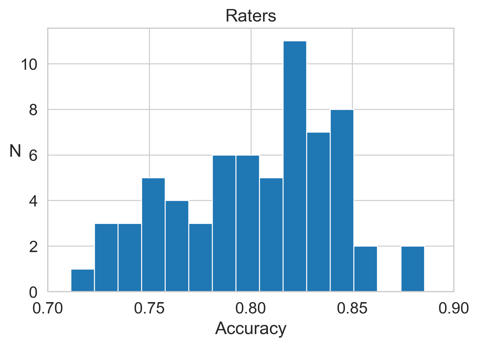
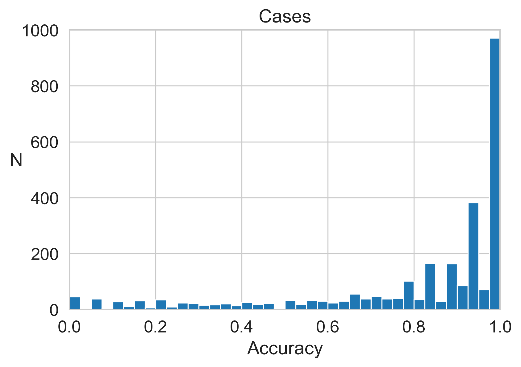
The description of the problem implies that cases have an inherent unknown "difficulty", which impacts the probability of a case being correctly classified by a rater, and that raters have a "skill" level with a similar effect. Modeling this therefore amounts to choosing some function that relates the success probability to those parameters. There are many possible ways of choosing such a function, a simple one might be:
$$P(\text{success}|\theta_n,\phi_m) = \frac{1+\theta_n\phi_m}{2}.$$
Here, $0<\theta_n<1$ is the difficulty level, $\theta_n=0$ being the most difficult, such that the best any rater can achieve is just a random choice ($P=1/2$). $0<\phi_m<1$ is similarly the skill level, such that the most skillful rater ($\phi_m=1$) can correctly classify the most easy cases with a 100% probability.
With the data $x_{nm}$ as described in the question ($x_{nm}=1$ for correct classification, $x_{nm}=-1$ for incorrect classification and $x_{nm}=0$ for no classification) the log-likelihood is (up to an irrelevant constant):
$$ \log \mathcal L = \sum_{n,m} \log(1 + x_{nm}\theta_n \phi_m)$$
and this can be maximized numerically (e.g. using gradient descent) in order to find the maximum likelihood estimators.
Notice that if we can assume that $\theta_n \phi_m \ll 1$, then the likelihood simplifies to
$$ \log \mathcal L \approx \sum_{n,m} x_{nm}\theta_n \phi_m \equiv \mathbf \theta^T X \mathbf \phi .$$
For vectors $\theta,\phi$ with fixed norms, this is maximized by the singular vectors that correspond to the largest singular value of the matrix $X$. So, an approximate solution can be achieved this way simply by performing a singular value decomposition of $X$.
More generally, we can write the likelihood as
$$ \log \mathcal L = \sum_{n,m} \log\left(\frac{1-x_{nm}}{2} + x_{nm}P_{nm}\right)$$
Where $P_{nm}$ is the success probability. (Notice that the expression inside the logarithm is equal to $P_{nm}$ when $x_{nm}=1$, $(1-P_{nm})$ when $x_{nm}=-1$, and a constant when $x_{nm}=0$). For a model that allow the probability to be zero, we can consider $P_{nm}=\theta_n \phi_m$ or, using unconstrained parameters, $P_{nm}=\text{Sigmoid}(w_n+v_m)=(1+e^{-(w_n+v_m)})^{-1}$. The corresponding modifications to the Python code are:
return -torch.log((1-X)/2 + teta * X * phi.T).sum()
or
return -torch.log((1-X)/2 + X * torch.sigmoid(w + v.T)).sum()
Comparing the maximum likelihood values of the two options with the provided data, we get a small but significant preference ($\Delta \log \mathcal L = 345.8$) for the second model. (The comparison is meaningful because the models have the same number of parameters). The MLE values for $v_m$ are: (converted to probabilities for case difficulty $w=0$)
print(torch.sigmoid(v).T)
tensor([[0.8846, 0.8338, 0.8891, 0.8149, 0.9040, 0.9188, 0.8654, 0.7761, 0.8773,
         0.8976, 0.9249, 0.8826, 0.8549, 0.9055, 0.9154, 0.9490, 0.7566, 0.8934,
         0.9529, 0.8855, 0.7359, 0.8765, 0.9106, 0.8981, 0.9141, 0.9172, 0.8148,
         0.9212, 0.8592, 0.8356, 0.8787, 0.9118, 0.8324, 0.9138, 0.8882, 0.9095,
         0.8305, 0.8393, 0.8893, 0.8384, 0.8906, 0.9201, 0.7997, 0.9011, 0.8896,
         0.9143, 0.9078, 0.9124, 0.9278, 0.8945, 0.7991, 0.7544, 0.9058, 0.8708,
         0.7664, 0.8078, 0.9104, 0.8673, 0.8346, 0.8012, 0.8408, 0.7689, 0.9018,
         0.8283, 0.8363, 0.8732]], grad_fn=<PermuteBackward0>)
Notice that, since the data is limited, not all differences between MLE values may be statistically significant. To determine that, further analysis of statistical significance is required.
Maximum likelihood implementation using PyTorch:
import torch

N, M = 3000, 70

#gererate random true parameters:
teta = torch.rand(N,1)
phi  = torch.rand(M,1)

#generate random data matrix X:
P = (1 + teta*phi.T)/2
X = 2*torch.bernoulli(P) - 1
#set about 70% of X entries to zero
X[torch.rand(N,M) > 0.3] = 0

#unconstrained optimization parameters,
#such that teta = sigmoid(w) and phi=sigmoid(v)
w = torch.randn(N,1,requires_grad=True)
v = torch.randn(M,1,requires_grad=True)

#likelihood loss function
def loss(w,v,X):
    teta = torch.sigmoid(w)
    phi = torch.sigmoid(v)
    return -torch.log(1 + teta * X * phi.T).sum()


optimizer = torch.optim.Adam([w,v],lr=0.05)

#gradient descent iterations
for iter in range(1000):
    optimizer.zero_grad()
    L = loss(w,v,X)
    L.backward()
    optimizer.step()


print('true phi:')
print(phi.T)
print('MLE:')
print(torch.sigmoid(v).T)
output:
true phi:
tensor([[0.1621, 0.4545, 0.1322, 0.9994, 0.4517, 0.4210, 0.5734, 0.9993, 0.8364,
         0.7181, 0.5347, 0.8723, 0.9996, 0.0760, 0.9831, 0.7306, 0.1410, 0.8279,
         0.2426, 0.5312, 0.6453, 0.3937, 0.9949, 0.1446, 0.1909, 0.2223, 0.0982,
         0.9986, 0.7534, 0.7858, 0.0199, 0.2229, 0.1371, 0.5162, 0.1269, 0.4183,
         0.7202, 0.9995, 0.0551, 0.7844, 0.0248, 0.0022, 0.2925, 0.9989, 0.0608,
         0.9984, 0.6897, 0.8560, 0.9992, 0.1023, 0.8478, 0.8740, 0.5565, 0.2198,
         0.9949, 0.5519, 0.8228, 0.3855, 0.3905, 0.4450, 0.3783, 0.3177, 0.8440,
         0.4595, 0.4974, 0.3771, 0.7208, 0.8438, 0.9292, 0.0892]],
       grad_fn=<PermuteBackward0>)
MLE:
tensor([[0.1528, 0.4522, 0.1803, 0.9994, 0.5803, 0.4260, 0.5195, 0.9988, 0.9986,
         0.6797, 0.4950, 0.9968, 0.9997, 0.0402, 0.9998, 0.7741, 0.1542, 0.9965,
         0.1423, 0.4255, 0.6306, 0.3968, 0.9996, 0.1225, 0.1858, 0.1826, 0.0672,
         0.9973, 0.9987, 0.9986, 0.0558, 0.2186, 0.1733, 0.4893, 0.0905, 0.4301,
         0.7361, 0.9985, 0.0657, 0.9991, 0.0501, 0.0018, 0.2379, 0.9986, 0.0548,
         0.9984, 0.6548, 0.9981, 0.9991, 0.1299, 0.7725, 0.9949, 0.5826, 0.2785,
         0.9995, 0.6145, 0.8397, 0.3643, 0.3875, 0.4685, 0.3267, 0.2936, 0.9969,
         0.5136, 0.5735, 0.3453, 0.6652, 0.9958, 0.9984, 0.1792]],
       grad_fn=<PermuteBackward0>)

 35% cases are correctly classified by all raters.