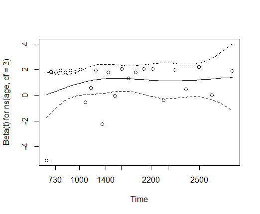
First, it's important to distinguish between the Schoenfeld residuals themselves and the score tests for trends of residuals over time that are used (starting with version 3 of the survival package) to evaluate deviations from proportional hazards (PH). Second, with respect to those score tests, it might be simpler to think about the tests on individual coefficients or on groups of coefficients (multiple-level categorical predictors, spline coefficients, etc) as special cases of the global test that's effectively done "under the hood" by cox.zph whether you ask for it or not. Third, the multiple residuals associated with a single predictor in the model can be combined with their associated regression-coefficient estimates to obtain the corresponding net residual in the linear predictor of the model.
Schoenfeld residuals
This page explains that
The Schoenfeld residuals are calculated for all covariates for each individual experiencing an event at a given time. Those are the differences between that individual's covariate values at the event time and the corresponding risk-weighted average of covariate values among all those then at risk.
If there are multiple coefficients associated with a predictor in a model, as in the situations you describe, there are multiple "covariates" in the above sense associated with that predictor, each with its own estimated regression coefficient.
The residuals are scaled inversely with respect to their covariances to get scaled Schoenfeld residuals $s^*_{k,j}$ for covariate $j$ at event time $t_k$. Grambsch and Therneau showed that the expected value of that residual is the difference between the time-fixed Cox-model coefficient estimate $\hat\beta_j$ and a potentially time-varying coefficient value at that event time:
$$E(s_{k,j}^*) + \hat \beta_j \approx \beta_j(t_k).$$
If PH holds, $\beta_j$ is constant over time. In that case, there should be no trend of those residuals over time.
Score tests for trends
Section 6.2 of the Therneau and Grambsch text explains how to test whether there is evidence of time trends in coefficients that would be inconsistent with PH. First, define some transformation of time $g(t)$; that's the transform argument to cox.zph(). Then, for covariate $j$, evaluate the following regression of the residual-based $\beta_j(t)$ against that function of time:
$$\beta_j(t) = \beta_j + \theta_j(g(t)-\bar g_j) $$
where $\bar g_j $ is the mean of the transformed event times. Then, for the set of $p$ covariates:
The null hypothesis of proportional hazards corresponds to $\theta_j \equiv 0, j = 1, ... ,p.$
As Therneau and Grambsch explain, this isn't done with a regression model per se but rather with a set of calculations that leads to a multi-parameter score test of that joint hypothesis. The test statistic, evaluated against $\chi^2_p$, is based on the $p \times 1$ score vector $U$ and the $p \times p$ Fisher information matrix $I$ evaluated at the above null hypothesis: the quadratic form $U^T I^{-1} U$. That's the global test.
Once you have $U$ and $I$ you can perform tests on subsets of covariates or on individual covariates, by restricting the calculation of the test statistic to the corresponding elements of $U$ and $I$ and evaluating against $\chi^2$ with degrees of freedom equal to the number of coefficients involved. In that sense, the test reported for a multi-coefficient predictor is a special case of the global test based on the subset of coefficients associated with it, and that for an individual coefficient for such a predictor is a special case of the test on the subset.
Combined scaled Schoenfeld residuals
The (unscaled) Schoenfeld residuals are first calculated for each individual event time and covariate. When terms=TRUE, the set of residuals for each event time for a multi-coefficient predictor is then combined as the inner product of the corresponding residuals and Cox model regression coefficients. That puts together all the residuals associated with that predictor, for that individual at that event time, into their net effect on the overall linear predictor of the Cox model. I've annotated below the critical code, which you can see by typing cox.zph at the command prompt:
## unscaled Schoenfeld residuals for all covariates from Cox fit
## event times in rows, covariates in columns
sresid <- resid$schoen
## if any predictor, indexed by nterm, has >1 covariate
if (terms && any(sapply(asgn, length) > 1)) {
    temp <- matrix(0, ncol(sresid), nterm)
    for (i in 1:nterm) {
        j <- asgn[[i]]
        if (length(j) == 1)  ## single covariate
            temp[j, i] <- 1
        else temp[j, i] <- fit$coefficients[j] ## multiple covariates
    }
    sresid <- sresid %*% temp  ## the inner product
    ## some lines omitted
}
That's done before additional calculations including scaling the residuals, so you can't readily reproduce that by a doing a similar calculation on the reported scaled residuals.

