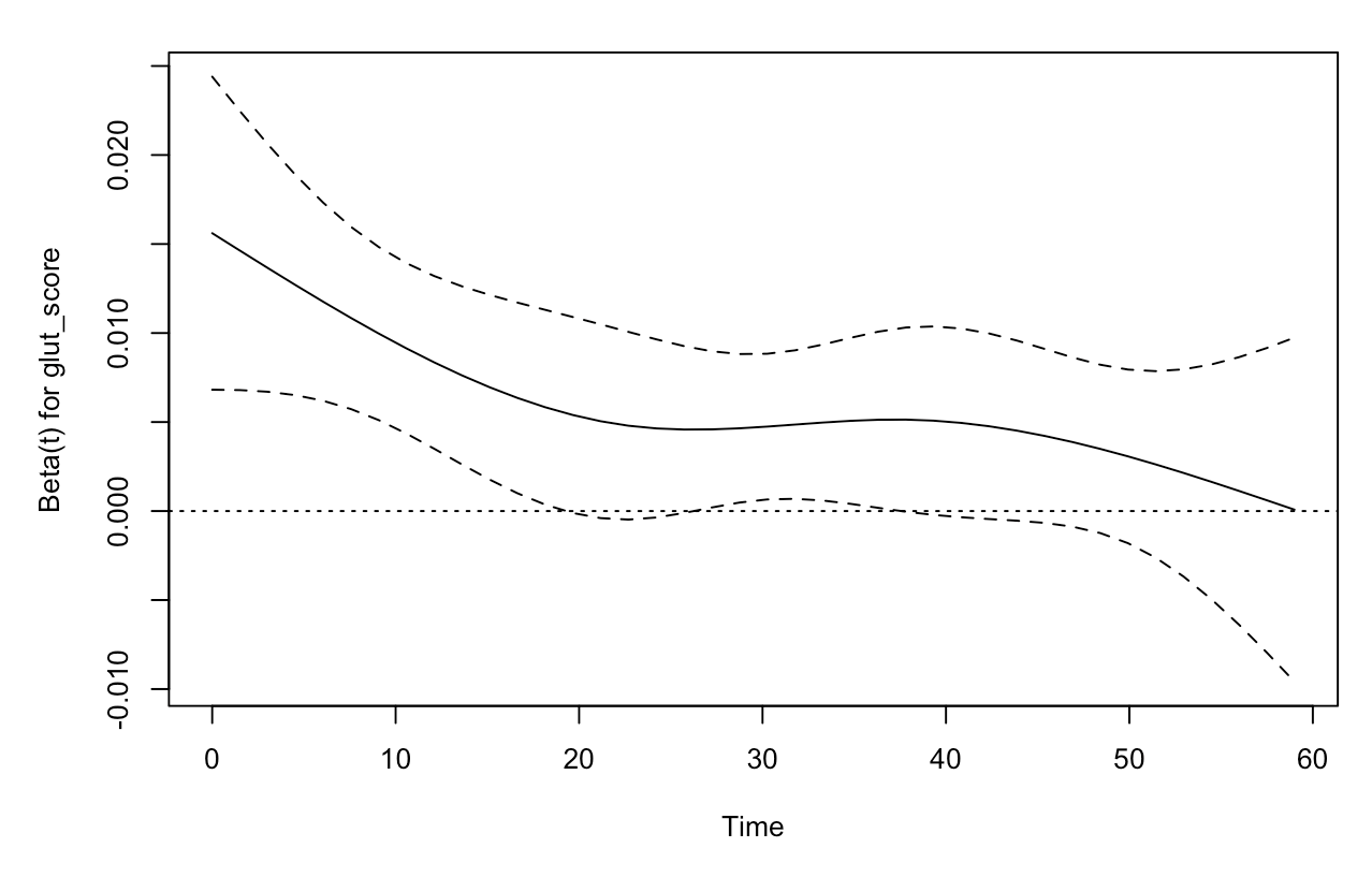
What's plotted starts with a variance-weighted transformation of the Schoenfeld residuals for a covariate, into what are called "scaled Schoenfeld residuals." Those are then added to the corresponding time-invariant coefficient estimate from the Cox model under the proportional hazards (PH) assumption and smoothed. The result is a plot of an estimate of the regression coefficient for the covariate over time. If the plot is reasonably flat, the PH assumption holds. Take this one step at a time.
Risk-weighted covariate averages and covariances
You start by determining, for each event time, the risk-weighted averages of covariate values and the corresponding risk-weighted covariance among covariate values over all individuals at risk at that time. That's essentially a part of the model-fitting process, anyway. The risks used for the weighting are simply the corresponding hazard ratios for the individuals at that time, the exponentiated linear-predictor values from the model.
Schoenfeld residuals
The Schoenfeld residuals are calculated for all covariates for each individual experiencing an event at a given time. Those are the differences between that individual's covariate values at the event time and the corresponding risk-weighted average of covariate values among all those then at risk. The word "residual" thus makes sense, as it's the difference between an observed covariate value and what you might have expected based on all those at risk at that time.
Scaled Schoenfeld residuals
The Schoenfeld residuals are then scaled inversely with respect to their (co)variances. The scaled values at an event time for an individual come from pre-multiplying the vector of original Schoenfeld residuals by the inverse of the corresponding risk-weighted covariate covariance matrix at that time.* You can think of this as down-weighting Schoenfeld residuals whose values are uncertain because of high variance.
The "plot of scaled Schoenfeld residuals"
Although the plot you show is generally called a "plot of scaled Schoenfeld residuals," that's not quite right.
The importance of the scaled Schoenfeld residuals comes from their associations with the time-dependence of a Cox regression coefficient. If $s_{k,j}^*$ is a scaled Schoenfeld residual for covariate $j$ at time $t_k$ and the estimated time-fixed Cox regression coefficient under PH is $\hat \beta_j$, then the expected value of $s_{k,j}^*$ is approximately the deviation of the actual coefficient value at time $t_k$, $\beta_j(t_k)$, from the PH-based estimate:
$$E(s_{k,j}^*) + \hat \beta_j \approx \beta_j(t_k).$$
That was shown by Grambsch and Therneau in 1994. The y-axis values of the plot for covariate $j$ are the sums of the scaled Schoenfeld residuals with the corresponding PH estimate $\hat \beta_j$.
Simple answer to the question
The smoothed plot is thus an estimate of the time dependence of the coefficient for the covariate $j$, $\beta_j(t_k)$. In your case, the plot indicates that your biomarker is most strongly associated with outcome at early times, dropping off to almost no association beyond a time value of 50-60.
The above is pretty much based on Therneau and Grambsch. Section 6.2 presents the plotting of scaled Schoenfeld residuals, with ordinary Schoenfeld residuals described in Section 4.6 and the formulas for risk-weighted covariate means and covariances in Section 3.1 (equations 3.5 and 3.7, respectively).
*The code in residuals.coxph() makes a simplifying assumption that the risk-weighted covariate covariance matrix is constant in time, and uses the average value. The inverse of that average risk-weighted covariate covariance matrix is then (conveniently) just the product of the coefficient covariance matrix times the number of events.

