Dealing with non-proportional hazards in a Cox model with many variables and a large dataset

Question

Summary: I am trying deal with non-proportional hazards in a Cox model on a large dataset. My question is whether the proportional hazards assumption really does not hold? If no, is the second model better? In the second model, can I interpret the hazard ratios as being averaged over the follow-up?

---

This is an observational cohort study. The goal is to identify covariates associated with misuse of a given prescription drug. Available covariates are patient's characteristics (e.g. sociodemographic characteritics, comorbidities, and exposure to other prescription drugs). With regard to data, all variables but misuse were assessed at inclusion. There is one row by patient for about 850,000 patients. The median time of follow-up is about 4 years. I am using R and the survival package.

summary(d)
#       id                time            misuse             age           privation         n_pharmacy     
#  Length:841161      Length:841161     Mode :logical   Min.   : 18.00   Min.   :-6.1055   Min.   :  1.000  
#  Class :character   Class :difftime   FALSE:798830    1st Qu.: 51.00   1st Qu.:-0.6641   1st Qu.:  1.000  
#  Mode  :character   Mode  :numeric    TRUE :42331     Median : 63.00   Median : 0.3707   Median :  1.000  
#                                                       Mean   : 62.53   Mean   : 0.2645   Mean   :  1.888  
#                                                       3rd Qu.: 75.00   3rd Qu.: 1.3357   3rd Qu.:  2.000  
#                                                       Max.   :108.00   Max.   : 8.5457   Max.   :490.000  
#                                                                                                           
#   n_prescriber       sex                 profession                      region       social_benefits
#  Min.   : 1.000   Women:487727   Employee     :684583   Other               :225913   Mode :logical  
#  1st Qu.: 1.000   Men  :353434   Student      : 61063   ILE DE FRANCE       :126893   FALSE:756037   
#  Median : 2.000                  Farmer       : 47756   AUVERGNE-RHONE-ALPES:103708   TRUE :85124    
#  Mean   : 2.037                  Self employed: 34938   NOUVELLE-AQUITAINE  : 82434                  
#  3rd Qu.: 3.000                  Other        : 12821   HAUTS-DE-FRANCE     : 79579                  
#  Max.   :98.000                                         OCCITANIE           : 77737                  
#                                                         (Other)             :144897                  
#  disease_diabetes disease_cancer   disease_psychosis disease_depression disease_bipolar  
#  Min.   :0.0000   Min.   :0.0000   Min.   :0.00000   Min.   :0.0000     Min.   :0.00000  
#  1st Qu.:0.0000   1st Qu.:0.0000   1st Qu.:0.00000   1st Qu.:0.0000     1st Qu.:0.00000  
#  Median :0.0000   Median :0.0000   Median :0.00000   Median :0.0000     Median :0.00000  
#  Mean   :0.2138   Mean   :0.1194   Mean   :0.01434   Mean   :0.1056     Mean   :0.01433  
#  3rd Qu.:0.0000   3rd Qu.:0.0000   3rd Qu.:0.00000   3rd Qu.:0.0000     3rd Qu.:0.00000  
#  Max.   :1.0000   Max.   :1.0000   Max.   :1.00000   Max.   :1.0000     Max.   :1.00000  
#                                                                                          
#  drug_antidepressants drug_antipsychotics drug_anxiolytics drug_hypnotics   disease_sclerosis
#  Min.   :0.0000       Min.   :0.00000     Min.   :0.00     Min.   :0.0000   Min.   :0.00000  
#  1st Qu.:0.0000       1st Qu.:0.00000     1st Qu.:0.00     1st Qu.:0.0000   1st Qu.:0.00000  
#  Median :0.0000       Median :0.00000     Median :0.00     Median :0.0000   Median :0.00000  
#  Mean   :0.2921       Mean   :0.04965     Mean   :0.29     Mean   :0.1554   Mean   :0.01068  
#  3rd Qu.:1.0000       3rd Qu.:0.00000     3rd Qu.:1.00     3rd Qu.:0.0000   3rd Qu.:0.00000  
#  Max.   :1.0000       Max.   :1.00000     Max.   :1.00     Max.   :1.0000   Max.   :1.00000  
#                                                                                              
#  disease_epilepsy drug_analgesics 
#  Min.   :0.000    Min.   :0.0000  
#  1st Qu.:0.000    1st Qu.:0.0000  
#  Median :0.000    Median :1.0000  
#  Mean   :0.012    Mean   :0.5921  
#  3rd Qu.:0.000    3rd Qu.:1.0000  
#  Max.   :1.000    Max.   :1.0000  
# 

Here is the initial model. As per @LukasLohse and @EdM comments, I used pspline() rather than binning the continuous variables.

(mod1 <- coxph(
  Surv(time, misuse) ~ sex + profession + region + social_benefits +
    pspline(age) + disease_diabetes + disease_cancer + disease_psychosis +
    disease_depression + disease_bipolar + drug_antidepressants +
    drug_antipsychotics + drug_anxiolytics + drug_hypnotics +
    disease_sclerosis + disease_epilepsy + drug_analgesics +
    pspline(privation) + pspline(n_pharmacy) + pspline(n_prescriber),
  d))
# Call:
# coxph(formula = Surv(time, misuse) ~ sex + profession + region + 
#     social_benefits + pspline(age) + disease_diabetes + disease_cancer + 
#     disease_psychosis + disease_depression + disease_bipolar + 
#     drug_antidepressants + drug_antipsychotics + drug_anxiolytics + 
#     drug_hypnotics + disease_sclerosis + disease_epilepsy + drug_analgesics + 
#     pspline(privation) + pspline(n_pharmacy) + pspline(n_prescriber), 
#     data = d)
# 
#                                  coef    se(coef)         se2       Chisq   DF                    p
# sexMen                       0.545716    0.010023    0.010021 2964.290300 1.00 < 0.0000000000000002
# professionStudent           -0.099402    0.021661    0.021651   21.058781 1.00   0.0000044540698675
# professionFarmer            -0.142702    0.027177    0.027173   27.570349 1.00   0.0000001514832404
# professionSelf employed      0.000875    0.023642    0.023639    0.001370 1.00               0.9705
# professionOther             -0.088560    0.049588    0.049586    3.189530 1.00               0.0741
# regionAUVERGNE-RHONE-ALPE   -0.088193    0.018958    0.018941   21.640550 1.00   0.0000032882603530
# regionHAUTS-DE-FRANCE        0.095135    0.020489    0.020459   21.559064 1.00   0.0000034309730169
# regionNOUVELLE-AQUITAINE    -0.105319    0.021587    0.021559   23.802937 1.00   0.0000010671950186
# regionGRAND-EST              0.183865    0.019956    0.019936   84.886836 1.00 < 0.0000000000000002
# regionOCCITANIE             -0.095754    0.020865    0.020839   21.060318 1.00   0.0000044504986112
# regionPROVENCE-ALPES-COTE   -0.020433    0.020784    0.020733    0.966560 1.00               0.3255
# regionOther                 -0.232146    0.017208    0.017182  181.998272 1.00 < 0.0000000000000002
# social_benefitsTRUE          0.435264    0.012578    0.012569 1197.572379 1.00 < 0.0000000000000002
# pspline(age), linear        -0.029874    0.000358    0.000357 6960.769812 1.00 < 0.0000000000000002
# pspline(age), nonlin                                           523.322648 3.08 < 0.0000000000000002
# disease_diabetes             0.066014    0.013020    0.013008   25.708530 1.00   0.0000003970681820
# disease_cancer               0.352342    0.015612    0.015601  509.368586 1.00 < 0.0000000000000002
# disease_psychosis            0.177948    0.031791    0.031784   31.330546 1.00   0.0000000217628522
# disease_depression          -0.049034    0.017719    0.017716    7.657802 1.00               0.0057
# disease_bipolar              0.094265    0.035887    0.035886    6.899421 1.00               0.0086
# drug_antidepressants         0.099505    0.012120    0.012117   67.404414 1.00 < 0.0000000000000002
# drug_antipsychotics          0.110140    0.021771    0.021768   25.594385 1.00   0.0000004212634991
# drug_anxiolytics             0.094379    0.011843    0.011842   63.505999 1.00   0.0000000000000016
# drug_hypnotics               0.163822    0.013496    0.013494  147.348442 1.00 < 0.0000000000000002
# disease_sclerosis            0.217410    0.038450    0.038447   31.971278 1.00   0.0000000156469032
# disease_epilepsy             0.180250    0.035848    0.035839   25.283294 1.00   0.0000004949772664
# drug_analgesics              0.197741    0.010393    0.010391  361.996372 1.00 < 0.0000000000000002
# pspline(privation), linea    0.005340    0.003348    0.003347    2.544280 1.00               0.1107
# pspline(privation), nonli                                       48.315245 3.02   0.0000000001882724
# pspline(n_pharmacy), line    0.008475    0.000804    0.000778  111.102269 1.00 < 0.0000000000000002
# pspline(n_pharmacy), nonl                                     3957.757338 3.00 < 0.0000000000000002
# pspline(n_prescriber), li    0.009743    0.003403    0.003206    8.196964 1.00               0.0042
# pspline(n_prescriber), no                                     5513.778770 3.00 < 0.0000000000000002
# 
# Iterations: 10 outer, 35 Newton-Raphson
#      Theta= 0.998 
#      Theta= 0.995 
#      Theta= 0.856 
#      Theta= 0.933 
# Degrees of freedom for terms= 1.0 4.0 7.0 1.0 4.1 1.0 1.0 1.0 1.0 1.0 1.0 1.0 1.0 1.0 1.0 1.0 1.0 4.0 4.0 4.0 
# Likelihood ratio test=41297  on 41.1 df, p=<0.0000000000000002
# n= 841161, number of events= 42331 

First, I checked the test for the proportional hazards assumption. The test yields significant p values for all variables except drug_hypnotics and privation.

(zph <- cox.zph(mod1))
#                         chisq    df                    p
# sex                    115.66  1.00 < 0.0000000000000002
# profession              82.42  4.00 < 0.0000000000000002
# region                 246.73  6.99 < 0.0000000000000002
# social_benefits        640.90  1.00 < 0.0000000000000002
# pspline(age)           671.35  4.08 < 0.0000000000000002
# disease_diabetes       243.78  1.00 < 0.0000000000000002
# disease_cancer          54.27  1.00     0.00000000000017
# disease_psychosis      113.22  1.00 < 0.0000000000000002
# disease_depression      10.96  1.00              0.00093
# disease_bipolar          6.53  1.00              0.01060
# drug_antidepressants     7.05  1.00              0.00793
# drug_antipsychotics    101.02  1.00 < 0.0000000000000002
# drug_anxiolytics        25.36  1.00     0.00000047614759
# drug_hypnotics           2.48  1.00              0.11524
# disease_sclerosis       48.00  1.00     0.00000000000427
# disease_epilepsy         6.23  1.00              0.01254
# drug_analgesics         20.42  1.00     0.00000620721265
# pspline(privation)       2.21  4.02              0.69915
# pspline(n_pharmacy)     98.71  4.00 < 0.0000000000000002
# pspline(n_prescriber)  758.89  4.00 < 0.0000000000000002
# GLOBAL                3025.73 41.08 < 0.0000000000000002

However, I learned that the test for the proportional hazards assumption may be too sensitive with large datasets. So, I ran the model and the test on samples of the dataset from 5,000 to 500,000 rows. The test yields mainly non-significant p values for the smaller datasets and the p values decrease with bigger dataset. So I wonder if the proportional hazards assumption really does not hold.

sizes <- c(5e3, 1e4, 5e4, 1e5, 5e5)
lapply(
  sizes,
  function(x) {
    set.seed(123)
    d_sample <- d[sample(nrow(d), x), ]
    mod_sample <- coxph(
      Surv(time, misuse) ~ sex + profession + region + social_benefits +
        pspline(age) + disease_diabetes + disease_cancer + disease_psychosis +
        disease_depression + disease_bipolar + drug_antidepressants +
        drug_antipsychotics + drug_anxiolytics + drug_hypnotics +
        disease_sclerosis + disease_epilepsy + drug_analgesics +
        pspline(privation) + pspline(n_pharmacy) + pspline(n_prescriber),
      d_sample)
    cox.zph(mod_sample)
  }
)
# [[1]]
#                          chisq    df    p
# sex                    1.13975  1.00 0.28
# profession             7.69648  3.99 0.10
# region                10.44668  6.96 0.16
# social_benefits        1.72961  1.00 0.19
# pspline(age)           2.65965  4.09 0.63
# disease_diabetes       0.69185  1.00 0.40
# disease_cancer         0.38253  1.00 0.53
# disease_psychosis      0.00826  0.99 0.93
# disease_depression     1.31969  1.00 0.25
# disease_bipolar        2.40380  1.00 0.12
# drug_antidepressants   4.71191  1.00 0.03
# drug_antipsychotics    0.19763  1.00 0.66
# drug_anxiolytics       0.18541  1.00 0.67
# drug_hypnotics         0.14610  1.00 0.70
# disease_sclerosis      0.15711  1.00 0.69
# disease_epilepsy       0.32902  1.00 0.57
# drug_analgesics        0.63544  1.00 0.42
# pspline(privation)     0.99400  4.09 0.92
# pspline(n_pharmacy)    0.04013  4.04 1.00
# pspline(n_prescriber)  6.96848  3.94 0.13
# GLOBAL                46.77002 41.07 0.25
# 
# [[2]]
#                            chisq    df      p
# sex                    1.7324310  1.00 0.1875
# profession             1.1127875  4.00 0.8919
# region                17.6495216  6.98 0.0135
# social_benefits       10.2481166  1.00 0.0014
# pspline(age)           6.0959077  4.09 0.2011
# disease_diabetes       0.7973985  1.00 0.3706
# disease_cancer         0.1911010  1.00 0.6612
# disease_psychosis      0.0000543  1.00 0.9940
# disease_depression     6.0284032  1.00 0.0140
# disease_bipolar        1.8739201  1.00 0.1707
# drug_antidepressants   5.8179192  1.00 0.0158
# drug_antipsychotics    2.1719878  1.00 0.1402
# drug_anxiolytics       0.1340706  1.00 0.7135
# drug_hypnotics         1.0893618  1.00 0.2961
# disease_sclerosis      0.0052149  1.00 0.9416
# disease_epilepsy       0.7470296  1.00 0.3859
# drug_analgesics        2.4016308  1.00 0.1210
# pspline(privation)     0.2374771  4.08 0.9942
# pspline(n_pharmacy)    0.2485274  4.00 0.9929
# pspline(n_prescriber)  8.6693439  4.01 0.0703
# GLOBAL                63.2622111 41.12 0.0148
# 
# [[3]]
#                          chisq    df                    p
# sex                     0.7090  1.00              0.39960
# profession              0.8557  4.00              0.93070
# region                 27.1760  6.98              0.00031
# social_benefits        37.3630  1.00        0.00000000097
# pspline(age)           36.4309  4.06        0.00000025522
# disease_diabetes       17.8586  1.00        0.00002366128
# disease_cancer          0.3343  1.00              0.56249
# disease_psychosis      12.3964  0.99              0.00042
# disease_depression      3.4480  1.00              0.06321
# disease_bipolar         1.9430  1.00              0.16324
# drug_antidepressants    0.8317  1.00              0.36133
# drug_antipsychotics    12.8328  1.00              0.00034
# drug_anxiolytics        1.3727  1.00              0.24110
# drug_hypnotics          0.0575  1.00              0.81026
# disease_sclerosis       4.2918  1.00              0.03822
# disease_epilepsy        0.2609  1.00              0.60917
# drug_analgesics         0.9306  1.00              0.33449
# pspline(privation)      1.5666  4.05              0.82030
# pspline(n_pharmacy)     0.0298  4.00              0.99989
# pspline(n_prescriber)  31.9281  4.01        0.00000199347
# GLOBAL                183.1964 41.07 < 0.0000000000000002
# 
# [[4]]
#                          chisq    df                    p
# sex                     8.4254  1.00              0.00370
# profession             10.7623  4.00              0.02933
# region                 26.3484  6.99              0.00043
# social_benefits        90.8523  1.00 < 0.0000000000000002
# pspline(age)           74.2570  4.07   0.0000000000000032
# disease_diabetes       45.6964  1.00   0.0000000000137271
# disease_cancer          1.9400  1.00              0.16331
# disease_psychosis       8.7727  1.00              0.00305
# disease_depression      6.6289  1.00              0.01002
# disease_bipolar         1.1974  1.00              0.27379
# drug_antidepressants    0.0882  1.00              0.76615
# drug_antipsychotics     9.6695  1.00              0.00187
# drug_anxiolytics        2.8865  1.00              0.08927
# drug_hypnotics          0.0712  1.00              0.78952
# disease_sclerosis       4.9664  1.00              0.02583
# disease_epilepsy        0.4901  1.00              0.48378
# drug_analgesics         0.4864  1.00              0.48532
# pspline(privation)      0.1099  4.05              0.99868
# pspline(n_pharmacy)     2.3126  4.00              0.67847
# pspline(n_prescriber)  87.0544  4.00 < 0.0000000000000002
# GLOBAL                370.1726 41.10 < 0.0000000000000002
# 
# [[5]]
#                          chisq    df                    p
# sex                     64.036  1.00   0.0000000000000012
# profession              34.024  4.00   0.0000007354678095
# region                 157.806  6.99 < 0.0000000000000002
# social_benefits        404.818  1.00 < 0.0000000000000002
# pspline(age)           405.226  4.04 < 0.0000000000000002
# disease_diabetes       150.054  1.00 < 0.0000000000000002
# disease_cancer          25.417  1.00   0.0000004603621634
# disease_psychosis       75.583  1.00 < 0.0000000000000002
# disease_depression      10.085  1.00              0.00149
# disease_bipolar          1.509  1.00              0.21929
# drug_antidepressants     1.613  1.00              0.20390
# drug_antipsychotics     69.617  1.00 < 0.0000000000000002
# drug_anxiolytics        18.988  1.00   0.0000131442043901
# drug_hypnotics           3.570  1.00              0.05883
# disease_sclerosis       25.672  1.00   0.0000004046233024
# disease_epilepsy         2.080  1.00              0.14906
# drug_analgesics         12.940  1.00              0.00032
# pspline(privation)       0.902  4.02              0.92542
# pspline(n_pharmacy)     29.935  4.00   0.0000050446453514
# pspline(n_prescriber)  394.932  4.00 < 0.0000000000000002
# GLOBAL                1771.473 41.04 < 0.0000000000000002
# 

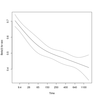
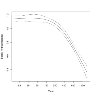
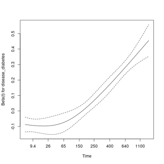
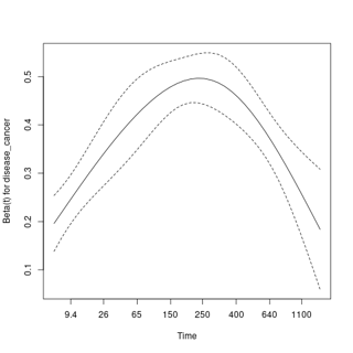
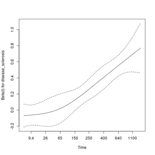
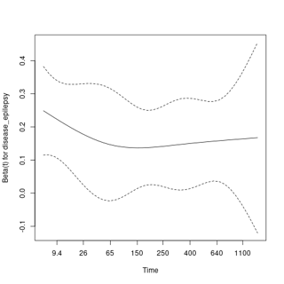
Second, I checked the plots of scaled Schoenfeld residuals. According to ?cox.zph, "The plot gives an estimate of the time-dependent coefficient $\beta(t)$. If the proportional hazards assumption holds then the true $\beta(t)$ function would be a horizontal line." I tried to find out whether the smoothed curves are "flat enough" (i.e. no obvious trend, but not necessarily around zero). However, I have no idea if it is the case and it seems quite subjective. I used resid = FALSE, otherwise the plots are less readable with so many observations due to overplotting and wider y-axis. Here is a selection of plots for some of the variables I am most interested in:

plot(zph[c(1, 5:7, 15:16)], resid = FALSE)

Finally, I tried to improve the model by:

• Stratifying on profession and region using strata() because I can do without hazard ratios for these variables if I really have to. Also, they have respectively 5 and 8 levels so I guess it can be problematic.
• Computing robust estimates using robust = TRUE to get averaged hazard ratios. There are several discussions on this topic on this site. However, it may not be relevant if non-proportional hazards is too strong (e.g. crossing curves).
• For the record, I also tested: (i) to compute hazard ratios per 6-month period using survSplit() but it seemed barely interpretable because of the high number of variables and time intervals; and (ii) to compute time-dependent covariates using coxph(... ~ ... + tt(...), ..., tt = ...) but I ran out of memory.

Here is the final model and the corresponding test for the proportional hazards assumption. However, I am not sure if it is really better than the initial model. Also, I am not sure if it is reasonable to interpret the hazard ratios as averaged hazard ratios here.

(mod2 <- update(
  mod1,
  . ~ . - profession + strata(profession) - region + strata(region),
  robust = TRUE
))
# Call:
# coxph(formula = Surv(time, misuse) ~ sex + social_benefits + 
#     pspline(age) + disease_diabetes + disease_cancer + disease_psychosis + 
#     disease_depression + disease_bipolar + drug_antidepressants + 
#     drug_antipsychotics + drug_anxiolytics + drug_hypnotics + 
#     disease_sclerosis + disease_epilepsy + drug_analgesics + 
#     pspline(privation) + pspline(n_pharmacy) + pspline(n_prescriber) + 
#     strata(profession) + strata(region), data = d, robust = TRUE)
# 
#                                  coef    se(coef)         se2       Chisq   DF                    p
# sexMen                       0.544878    0.010052    0.010022 2938.213957 1.00 < 0.0000000000000002
# social_benefitsTRUE          0.433589    0.012602    0.012582 1183.751417 1.00 < 0.0000000000000002
# pspline(age), linear        -0.030315    0.000353    0.000359 7356.835050 1.00 < 0.0000000000000002
# pspline(age), nonlin                                           718.483092 3.08 < 0.0000000000000002
# disease_diabetes             0.066262    0.013079    0.013010   25.666588 1.00   0.0000004057922648
# disease_cancer               0.353056    0.015577    0.015601  513.700565 1.00 < 0.0000000000000002
# disease_psychosis            0.175065    0.033519    0.031795   27.278811 1.00   0.0000001761309658
# disease_depression          -0.048150    0.018199    0.017714    7.000028 1.00               0.0082
# disease_bipolar              0.094382    0.036487    0.035888    6.691208 1.00               0.0097
# drug_antidepressants         0.100197    0.012491    0.012117   64.345364 1.00   0.0000000000000010
# drug_antipsychotics          0.110181    0.022501    0.021770   23.978708 1.00   0.0000009740698818
# drug_anxiolytics             0.093696    0.012070    0.011843   60.260027 1.00   0.0000000000000083
# drug_hypnotics               0.164276    0.013789    0.013495  141.931859 1.00 < 0.0000000000000002
# disease_sclerosis            0.217979    0.038253    0.038449   32.470871 1.00   0.0000000120992518
# disease_epilepsy             0.182080    0.036574    0.035838   24.784321 1.00   0.0000006411690271
# drug_analgesics              0.197617    0.010429    0.010393  359.044502 1.00 < 0.0000000000000002
# pspline(privation), linea    0.004665    0.003408    0.003429    1.874066 1.00               0.1710
# pspline(privation), nonli                                       60.198659 3.02   0.0000000000005512
# pspline(n_pharmacy), line    0.006325    0.000414    0.001191  233.189091 1.00 < 0.0000000000000002
# pspline(n_pharmacy), nonl                                     4117.244575 3.00 < 0.0000000000000002
# pspline(n_prescriber), li   -0.002231    0.001509    0.009633    2.184200 1.00               0.1394
# pspline(n_prescriber), no                                     6139.301123 3.00 < 0.0000000000000002
# 
# Iterations: 10 outer, 33 Newton-Raphson
#      Theta= 0.998 
#      Theta= 0.995 
#      Theta= 0.857 
#      Theta= 0.934 
# Degrees of freedom for terms= 1.0 1.0 4.1 1.0 1.0 1.0 1.0 1.0 1.0 1.0 1.0 1.0 1.0 1.0 1.0 4.0 4.0 4.0 
# Likelihood ratio test=39343  on 30.1 df, p=<0.0000000000000002
# n= 841161, number of events= 42331 

cox.zph(mod2)
#                         chisq    df                    p
# sex                    118.12  1.00 < 0.0000000000000002
# social_benefits        557.47  1.00 < 0.0000000000000002
# pspline(age)           651.44  4.08 < 0.0000000000000002
# disease_diabetes       257.58  1.00 < 0.0000000000000002
# disease_cancer          48.13  1.00      0.0000000000040
# disease_psychosis       95.38  1.00 < 0.0000000000000002
# disease_depression       7.89  1.00               0.0050
# disease_bipolar          4.88  1.00               0.0271
# drug_antidepressants     6.75  1.00               0.0094
# drug_antipsychotics     87.50  1.00 < 0.0000000000000002
# drug_anxiolytics        22.70  1.00      0.0000018950800
# drug_hypnotics           3.20  1.00               0.0735
# disease_sclerosis       46.86  1.00      0.0000000000076
# disease_epilepsy         5.86  1.00               0.0154
# drug_analgesics         22.99  1.00      0.0000016238257
# pspline(privation)       2.73  4.02               0.6069
# pspline(n_pharmacy)    136.35  4.00 < 0.0000000000000002
# pspline(n_prescriber)  877.64  4.00 < 0.0000000000000002
# GLOBAL                2724.55 30.09 < 0.0000000000000002

Answer 1

As references from links in the question explain, if the proportional hazards (PH) assumption doesn't hold then a Cox regression coefficient (which is exponentiated to give the hazard ratio, HR) represents a type of average over the events. Provided that you use robust standard errors (as you do), you can perform inference, for example testing whether that "average" coefficient is different from 0 (HR different from 1). Stratification on variables that aren't of substantive interest, as in your second model, is a well accepted way to try to minimize PH violations. Having too few events per stratum (or per combination of strata) can be a problem in general, but shouldn't be in such a large data set.

A plot of scaled Schoenfeld residuals over time indicates the nature of the deviation from PH, its magnitude and shape over time. Yes, deciding whether a curve is "flat enough" is somewhat subjective, but it can be based on your understanding of the subject matter. Those plots can also provide information that can suggest reasons why the PH assumption might not hold.

Your example plots illustrate this nicely.

For example, the plot for disease_epilepsy has coefficients ranging from about 0.25 (HR, 1.28) to 0.17 (HR, 1.18). Based on your understanding of the subject matter, does that difference in HR matter in practice? I doubt it. You are probably safe to think of that being "flat enough" even though the cox.zph() result says that it has a "significant" deviation from PH. That's where the very large numbers of events comes into play; even a small deviation of no practical significance can then appear to be "significant."

The plot for disease_diabetes tells a completely different story. From your second model, its "average" coefficient value of 0.066 (HR, 1.07) doesn't seem to describe the results at all well. Its coefficient starts near -0.1 (HR, 0.9), stays about constant for two months, and then rises consistently to a value of about 0.4 (HR, 1.5). Such a change in HR over time seems to be substantively important. The plot for disease_sclerosis has a similar pattern.

The plot for sex drops over time, from a coefficient of 0.7 (HR, 2.0) to 0.4 (HR, 1.5). The "average" coefficient of 0.54 seems reliably to be different from zero. Does your understanding of the subject matter suggest any reasons why the male-female difference in misuse risk might drop over time?

The plot for the "age" spline remains high for about 6 months, then drops. Several of your other plots suggest changes in slope at 2 months. Might those represent durations of initial prescriptions, perhaps with early right censoring for those who came off prescriptions without misuse? Might that be informative censoring? Informative censoring would call into question the entire modeling process. You should at least examine the distributions of right-censoring times and event times. If there isn't much right censoring at the end of prescriptions, then those patterns might represent lack of later access to the drug unless an individual took the effort and risk to obtain it illegally.

I suspect that the plot for disease_cancer has to do with the course of that disease. The coefficient stays comfortably above 0 at all times but reaches a peak at about 1 year. I wonder if the drop at later times represents death as a competing risk.

Overall, it seems that "the proportional hazards assumption really does not hold" for at least some of the predictors in your model. You have to apply your understanding of the subject matter to decide how to deal with it, not only in the modeling but also in describing your results to others.