Power analysis for GAMM

Question

Question

I am struggling with understanding how to run a simulated power analysis for GAMMs. Though my planned studies will include more variables, the core issue I'm trying to work out is to simulate the following:

• A binary outcome y. However, since I don't know how to correlate y here, I have opted to just use a Gaussian response as it is easier to model.
• Two predictors, modeled with s(x, by = group) to estimate this for two groups.
• The variables should be moderately correlated, with x2 having a negative association with y.
• An interaction will be modeled as ti(x1,x2,by=group).
• Subject and item random effects (with no specific prior information).
• For Group 1, x1 and x2 should have a larger effect on y.

Code

The best I could come up with was something like this for a basic GAM:

#### Load Libraries #### 
library(mgcv)
library(tidyverse)
library(correlation)
library(faux)
set.seed(123)

#### Perform Simulation PA ####
B <- 10 # number of simulations (10 for now so its faster)
p1 <- NULL # store p values
p2 <- NULL
p3 <- NULL 
p4 <- NULL
p5 <- NULL 
p6 <- NULL

for (i in 1:B) {
  
  #### Create RE Grid ####
  sub <- factor(1:50)
  item <- factor(1:20)
  obs <- length(sub)*length(item)
  grid <- expand.grid(sub=sub,
                      item=item)
  
  #### Set Up Simulation Parameters ####
  n <- 50 # sample size
  alpha <- 0.05 # significance level
  power <- 0.8 # desired power
  
  #### Simulate Data ####
  dat <- rnorm_multi(n = n, 
                     mu = c(20, 20, 20),
                     sd = c(10, 10, 10),
                     r = c(0.30, 0, -.30), 
                     varnames = c("x1", "x2", "y"),
                     empirical = FALSE) 
  
  #### Make Grouping Factor ####
  group <- factor(
    rep(c(1,2),each=25),
    labels = c("Group 1", "Group 2")
  ) # not sure how to show differences in groups
  
  #### Merge Data ####
  df <- data.frame(dat,group,grid) %>% 
    as_tibble()
  df
  
  #### Build Model ####
  model_sim <- bam(y 
                   ~ s(x1, by = group)
                   + s(x2, by = group) 
                   + ti(x1,x2, by = group)
                   + s(sub, bs = "re")
                   + s(item, bs = "re"),
                   data = df) # fit GAM model to simulated data
  
  #### Store P Values ####
  p1[i] <- as.vector(summary(model_sim)$s.table[1,"p-value"])
  p2[i] <- as.vector(summary(model_sim)$s.table[2,"p-value"])
  p3[i] <- as.vector(summary(model_sim)$s.table[3,"p-value"])
  p4[i] <- as.vector(summary(model_sim)$s.table[4,"p-value"])
  p5[i] <- as.vector(summary(model_sim)$s.table[5,"p-value"])
  p6[i] <- as.vector(summary(model_sim)$s.table[6,"p-value"])
  
  p.data <- data.frame(p1,p2,p3,p4,p5,p6)
    }

#### Inspect P Values for Variables 1:6 ####
p.data

Problems

Running this as-is takes forever, even with the very small number of boots here $(B = 10)$ and often doesn't converge, with this error popping up:

Warning message:
In bgam.fitd(G, mf, gp, scale, nobs.extra = 0, rho = rho, coef = coef,  :
  algorithm did not converge

I'm assuming it has to do with the data I have simulated. I also have no way of getting the groups to do anything other than arbitrarily split, while tinkering sometimes leads to complete separation in the GAMM (which I obviously don't want). As mentioned in the Question section, one group should have a predictably larger effect on y for each x, so modeling this would be helpful, Finally, achieving all of this somehow with binary data seems hard, so I have no way of figuring that part out.

So to summarize, I need to solve the following:

• What is causing the slow/weird estimaton?
• How do I get the groups to have a meaningful distinction from each other?
• Is there a way to make the outcome data binary? This is not my greatest priority, but it would be a nice bonus.

Edit

(continuation of first edit)

Because I don't want to make this question verbose, I've only included my recent changes. To follow the advise in the comments (hopefully I've done that), I tried estimating $y$ in the way prescribed in the data simulation functions of mgcv and gratia. I have kept it simple and made one "positive" function that varies slightly by group and one "negative" function that varies slightly by group.

#### Load Libraries #### 
library(mgcv)
library(tidyverse)
library(gratia)
library(faux)

#### N and Scale ####
set.seed(123)
n <- 100
scale <- 1

#### Create X and F ####
x1 <- runif(n, 0, 1)
x2 <- runif(n, 0, 1)
f1.x1 <- exp(3 * x1) 
f2.x1 <- exp(2 * x1)
f1.x2 <- exp(3 * x2) * -1
f2.x2 <- exp(2 * x2) * -1 
e <- rnorm(n, 0, scale)

#### Create Factors ####
fac <- as.factor(sample(1:2,n,replace=TRUE))
fac.1 <- as.numeric(fac==1)
fac.2 <- as.numeric(fac==2)

#### Estimate Y ####
y <- x1 + x2 + f1.x1*fac.1 + f2.x1*fac.2 + f1.x2*fac.1 + f2.x2*fac.2 + e 

#### Merge Data ####
df <- data.frame(y=y, # y values
                 x1=x1, # x values
                 x2=x2,
                 fac=fac) # factors

#### Convert and Inspect ####
data <- df %>% 
  as_tibble()
data

#### Fit Model ####
fit <- gam(y
           ~ fac 
           + s(x1, by = fac)
           + s(x2, by = fac)
           + ti(x1, x2, by = fac),
           method = "REML",
           data = data)
summary(fit)
draw(fit)

Which gives me this:

This gets me close to what I want for now with the main effects and their grouping (though the error seems to always be higher for the second factor). The major parts I am still missing:

1. How do I code the interaction between the two main effects? I am aware of how you do this in a vanilla regression, but not GAMs. I've tried assembling functions to do this like ti.function <- function(x1,x2){x1*x2} into y, but this doesn't seem to do anything different. I also tried correlating the variables beforehand using this method, but this in turn changes the direction of the plotted function. To summarize, I need increases in $x_1$ to be associated with increases in $y$, increases in $x_2$ to be associated with decreases in $y$, and and a linear interaction between $x_1$ and $x_2$ When $x_1$ is high and $x_2$ is low, this should result in higher $y$.
2. I still don't know how to add in subject/item random variance in a meaningful way. The faux package seems promising, but so far my attempts to add REs have failed.
3. I'm having issues adjusting the error variance with the scale object in this simulation. The standard error seems to always be relatively low but I expect my actual data to have more, so I would like to have better ways to tweak this.

Another Edit...(Dec 2023)

TLDR: I have solved the perfect prediction issues and have included crossed random effects like I originally wanted, but the relationships between the predictors and outcome are still not ideal.

I have still not solved my problem after repeated attempts, so I am setting up another bounty. I realize part of my issue previously was not providing enough information about the variables. Unfortunately, there is a serious lack of a priori information for my case, so I can only fill in what I know from some work in my area. However, I can offer a lot more information based off some previous knowledge of the research and what previous answerers have suggested adding. The variables should have the following features:

• A binary dependent variable called RD for "reading success" with values $0$ for failure to read and $1$ for success.
• A group variable called LG for "language group", where the L1 group has a higher rate of reading success than the L2 group. Its unclear what this means from a logistic sense. In one analysis the L1 group scored a mean of $120/150$ items correct and the L2 group merely got $30/150$, but the L2 group came from a poor disadvantaged background. Another study only found a $15$ point difference in scores on average (with the L2 group again scoring lower), but the L2 group in this case was from a much higher SES group. The actual reading test is a scale which ranges from a total score of $[0,150]$.
• A discrete subject-level variable called OA which has a positive linear effect on RD for the L2 group and a more weak curvilinear effect for the L1 group. There does not appear to be strong differences between the groups in at least one study (L1 OA = $12/16$, L2 OA = $11/16$) but I imagine those differences also vary wildly in reality and I have a strong feeling that the differences are more extreme than what is reported in just one study. As one can see, the scores range between $[0, 16]$. However, another study uses a similar measure range between $[0,20]$ with reported scores of $11/20$ for the L2 group but no reported scores of L1 groups with this measure.
• A discrete item-level variable called GC which has a negative linear effect on reading for the L2 group and a more weak curvilinear effect for the L1 group. The mean of the GC variable should be about $115$ and has no ceiling value, so it spans the range $[0, \infty)$. A previous analysis showed that GC was linear for reading and curvilinear for writing for the L1 group, so to be careful I am just going to assume the relationship is generally curvilinear for the L1 group, but that is of course just an assumption.
• A subject x item crossed random effects design, with a starting estimate of $50$ subjects per group and $150$ reading items. However, because this is a power analysis, the items will be essentially fixed and I am only after the number of subjects required for adequate power.
• Something else to add is that the estimates are likely to be fairly noisy. In the previous simulations in my question and the generous answer by Gavin, the standard error is very narrow, but I anticipate that this will not be the case given how measures in my field are not strongly correlated with the response.

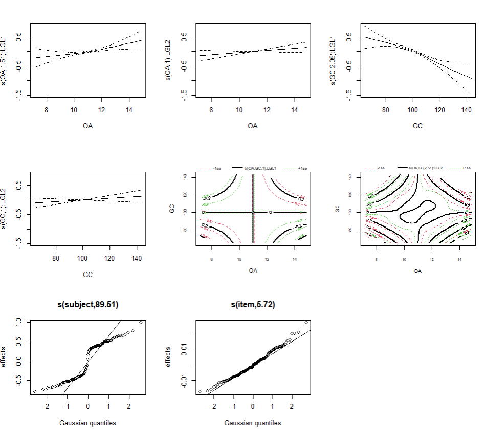
The only thing I have been able to do to modify the code so far is something like this, which at least includes the random effects and logistic regression I need (thus solving the perfect prediction issues and added in random effects like I needed before), but the simulation still doesn't model the data like I would hope. Note for simplicity I just included continuous versions of the predictors because I ran into some more issues with Poisson-distributed variables:

#### Load Libraries ####
library(tidyverse)
library(mgcv)

#### Set Seed ####
set.seed(123)

#### Define REs ####
n_subjects <- 100
n_items <- 150

#### Create Subject Data ####
subject_data <- data.frame(
  subject = rep(1:n_subjects, each = n_items),
  LG = rep(c("L1", "L2"), each = n_items * 50),
  OA = rnorm(n_subjects * n_items, mean = 11, sd = 1)
)

#### Create Item Data ####
item_data <- data.frame(
  item = rep(1:n_items, times = n_subjects),
  GC = rnorm(n_subjects * n_items, mean = 100, sd = 10)
)

#### Combine Data ####
data <- cbind(subject_data, item_data)
glimpse(data)

#### Define Y Variable ####
data$RD <- with(data, rbinom(n_subjects * n_items, 1, plogis(
  (LG == "L1") * (0.05 * OA - 0.0001 * GC^2) +
    (LG == "L2") * (0.03 * OA - 0.0001 * GC) +
    (LG == "L2") * (0.0002 * OA * GC)
)))

data.fix <- data %>% 
  mutate(subject = factor(subject),
         item = factor(item))

#### Fit GAMM ####
fit <- bam(
  RD
  ~ s(OA, by = LG)
  + s(GC, by = LG)
  + ti(OA, GC, by =LG)
  + s(subject, bs = "re")
  + s(item, bs = "re"),
  data=data.fix,
  family = binomial
)

#### Plot Effects ####
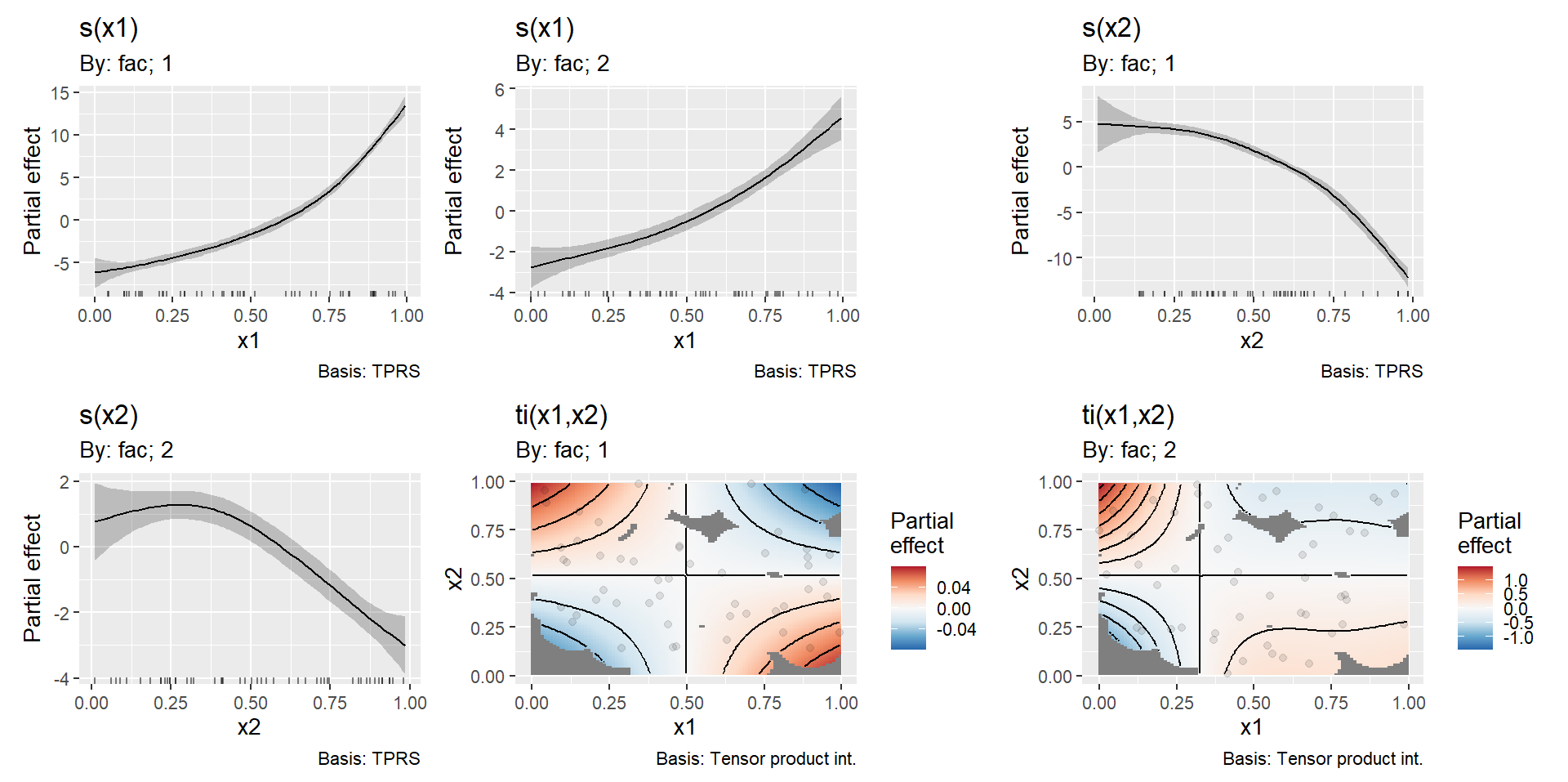
plot(fit,
     pages=1)

I'm not looking for an exact answer to my problem, so the solution doesn't need to fit all of these criteria exactly. I just need a workable logistic GAMM with crossed random effects, and if it achieves most of what I am trying to get here then I will be happy.

Answer 1

This is a work in progress...

---

Using your example:

#### Load packages #### 
library(mgcv)
library(dplyr)
library(gratia)
library(tibble)

#### N and Scale ####
set.seed(123)
n <- 100
scale <- 2

#### Create X and F ####
x1 <- runif(n, 0, 1)
x2 <- runif(n, 0, 1)
f1 <- function(x, b, c = 1) exp(b * x) * c
f2 <- function(x, b, c = 1) exp(b * x) * c
f1_x1 <- f1(x1, b = 3) 
f2_x1 <- f2(x1, b = 2)
f1_x2 <- f1(x2, b = 3, c = -1)
f2_x2 <- f2(x2, b = 2, c = -1)
e <- rnorm(n, 0, scale)

#### Create Factors ####
fac <- as.factor(sample(1:2,n,replace=TRUE))
fac1 <- as.numeric(fac==1)
fac2 <- as.numeric(fac==2)

#### Estimate Y ####
y <- x1 + x2 + f1_x1*fac1 + f2_x1*fac2 + f1_x2*fac1 + f2_x2*fac2 + 
     ((f1_x1*f1_x2) * fac1) + ((f2_x1*f2_x2) * fac2) + # interactions
     e 

#### Merge Data ####
df <- tibble(y = y, x1 = x1, x2 = x2, fac = fac)

Absent any information on the nature of the interactions, I simply created the interactions $f_{\text{fac}}(x_1,x_2)$ in the same way you'd create an interaction in a linear model, you multiply the values of the two predictors together, hence:

((f1_x1*f1_x2) * fac1) + ((f2_x1*f2_x2) * fac2)

#### Fit Model ####
fit <- gam(y ~ fac + s(x1, by = fac) + s(x2, by = fac) + ti(x1, x2, by = fac),
           method = "REML",
           data = df)

Now we get a significant pair of pure interaction tensor products:

summary(fit)

> summary(fit)                                                                

Family: gaussian 
Link function: identity 

Formula:
y ~ fac + s(x1, by = fac) + s(x2, by = fac) + ti(x1, x2, by = fac)

Parametric coefficients:
            Estimate Std. Error t value Pr(>|t|)    
(Intercept) -39.3796     0.5046  -78.05   <2e-16 ***
fac2         30.0963     0.5935   50.71   <2e-16 ***
---
Signif. codes:  0 ‘***’ 0.001 ‘**’ 0.01 ‘*’ 0.05 ‘.’ 0.1 ‘ ’ 1

Approximate significance of smooth terms:
                  edf Ref.df       F p-value    
s(x1):fac1      5.406  6.299  939.12  <2e-16 ***
s(x1):fac2      2.231  2.761   33.18  <2e-16 ***
s(x2):fac1      5.973  6.805 1260.83  <2e-16 ***
s(x2):fac2      3.451  4.194  138.91  <2e-16 ***
ti(x1,x2):fac1 11.600 13.004  358.29  <2e-16 ***
ti(x1,x2):fac2  4.154  5.728   23.10  <2e-16 ***
---
Signif. codes:  0 ‘***’ 0.001 ‘**’ 0.01 ‘*’ 0.05 ‘.’ 0.1 ‘ ’ 1

R-sq.(adj) =  0.997   Deviance explained = 99.8%
-REML = 245.19  Scale est. = 4.1068    n = 100

And we can inspect the fitted smooths with

draw(fit)

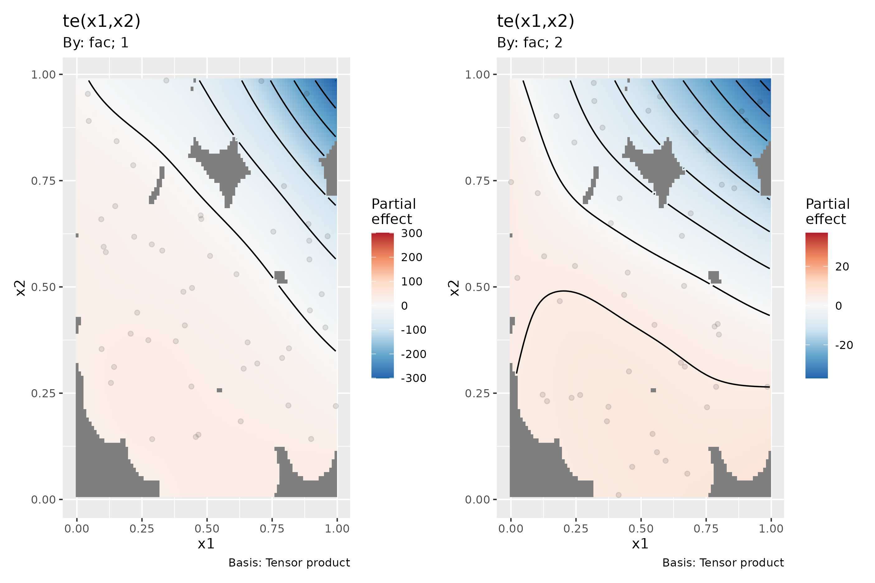
It can be hard to see if the estimated functions do what you want from that decomposed fit, so fitting with te() should help:

#### Fit Model ####
m <- gam(y ~ fac + te(x1, x2, by = fac),
         method = "REML", data = df)

draw(m)

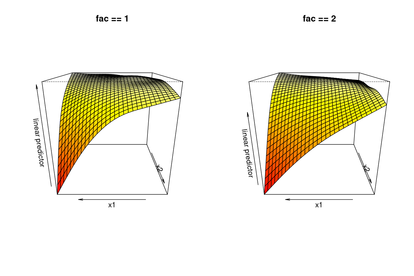
But you can also use vis.gam() from {mgcv} to visualise the estimated surfaces:

layout(matrix(c(1,2), ncol = 2))
vis.gam(m, view = c("x1", "x2"), theta = 180, phi = 20,
        cond = list(fac = 1), main = "fac == 1")
vis.gam(m, view = c("x1", "x2"), theta = 180, phi = 20,
        cond = list(fac = 2), main = "fac == 2")
layout(1)

which produces:

So the estimated functions fit the requirements, I believe.

To check all of this, you want to use regular data over the range of the covariates so that you can actually plot the true surfaces you are trying to estimate:

g1 <- g2 <- seq(0, 1, by = 0.01)
gg <- expand.grid(g1, g2)
f1f2 <- function(x1, x2, b = c(3,2), c = c(1,-1)) {

}

For example, f1 for x1:

g1 <- seq(0, 1, by = 0.01)
ggplot(data = data.frame(x = g1), aes(x)) + 
    geom_function(fun = f1, args = list(b = 3, c = 1))

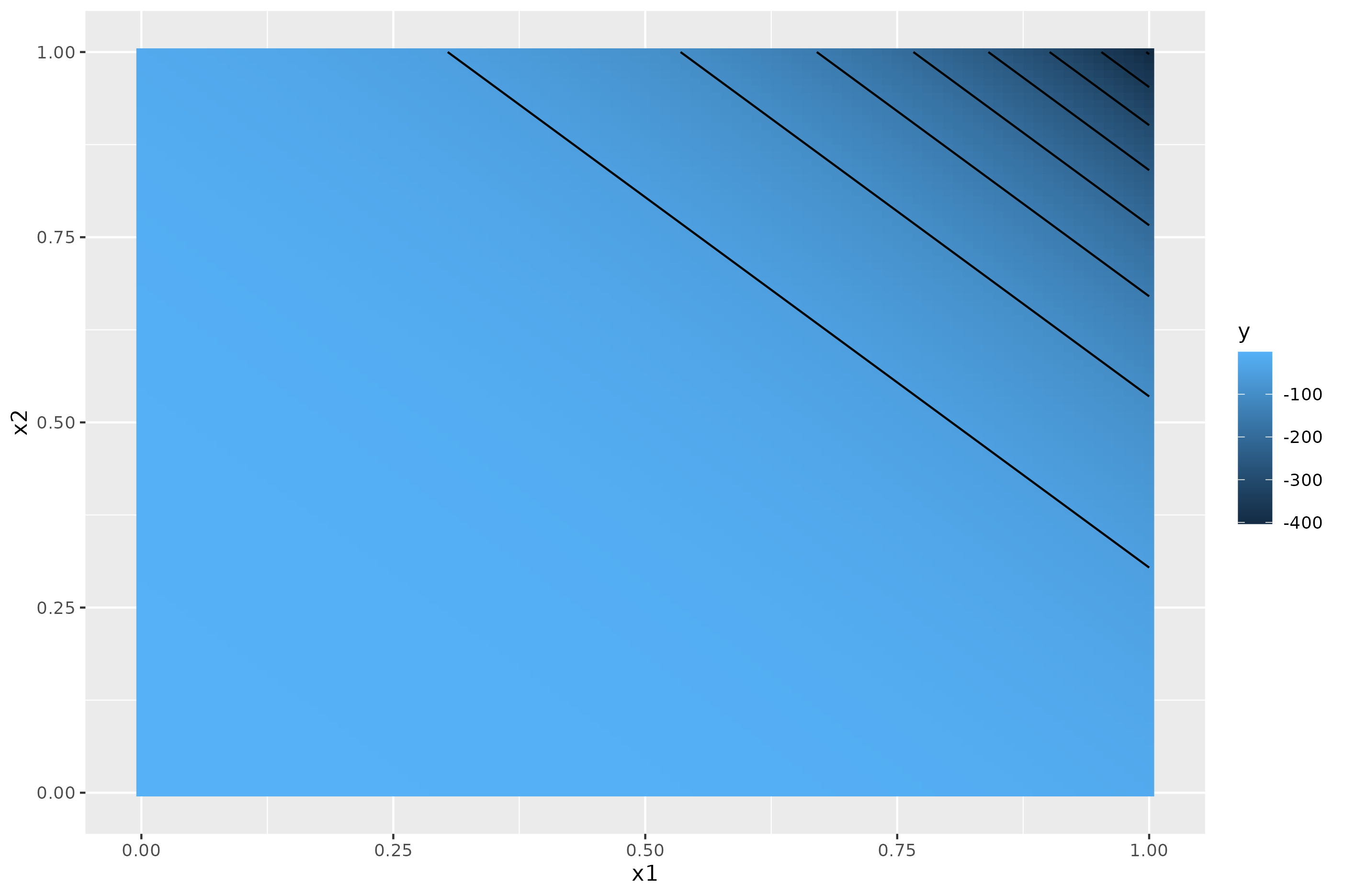
And this is the linear interaction of the two non-linear functions:

ff <- function(x, b) {
  f1_x1 <- f1(x[,1], b = b)
  f1_x2 <- f1(x[,2], b = b, c = -1)
  f1_x1 * f1_x2
}

gg <- expand.grid(x1 = g1, x2 = g1)
dt <- cbind(gg, y = ff(gg, b = 3))

ggplot(dt, aes(x = x1, y = x2)) + 
    geom_raster(aes(fill = y)) + 
    geom_contour(aes(z = y), colour = "black")

Or, for the full effect specified in the linear predictor

ff_full <- function(x, b) {
  f1_x1 <- f1(x[,1], b = b)
  f1_x2 <- f1(x[,2], b = b, c = -1)
  x[,1] + x[,2] + f1_x1 + f1_x1 + (f1_x1 * f1_x2)
}

gg <- expand.grid(x1 = g1, x2 = g1)
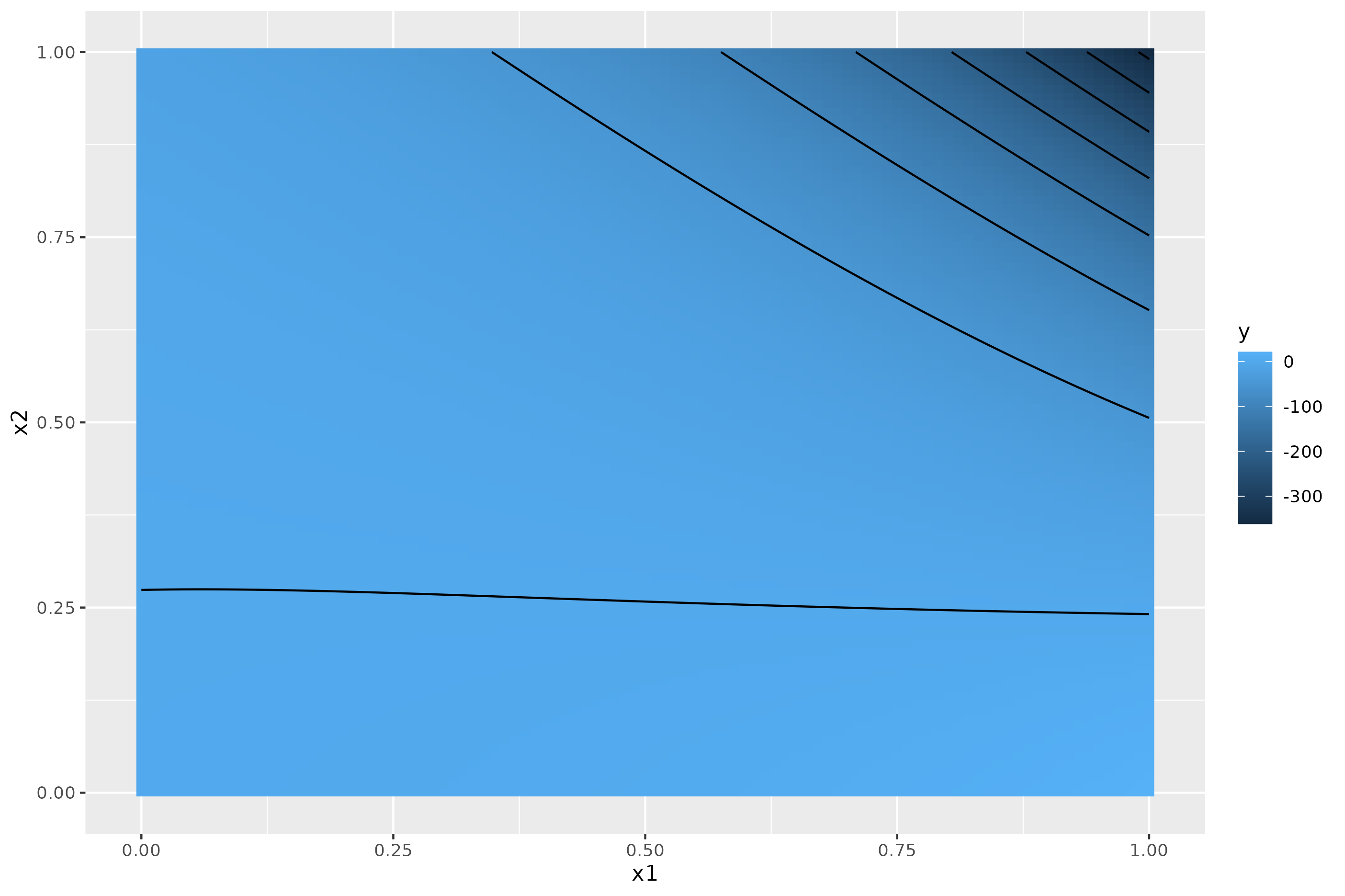
dt <- cbind(gg, y = ff_full(gg, b = 3))

ggplot(dt, aes(x = x1, y = x2)) + 
    geom_raster(aes(fill = y)) + 
    geom_contour(aes(z = y), colour = "black")

Being able to plot the truth (as I've done at the end (change the value of b in the creation of gg to get the second group)) is important and you should really start there so that you can get the shapes of the functions you anticipate correct. Then it is pretty simple to then simulate data from those functions and fit a model to them.

Simulating binary data

This becomes easier when you consider the form of a generalized linear model. There we would have

$$y_i \sim \text{Bernoulli}(\mu_i)$$

and

$$\text{logit}(\mu_i) = \eta_i$$

where $\mu_i$ is the expected value on the response scale (a probability that $y_i = 1$, give the value of $\eta_i$, the linear predictor, and $\text{logit}()$ is the canonical link function for the binomial GLM (of which the Bernoulli distribution is a special case).

There's no error term $\varepsilon$, your e in a GLM; the data are a random draw from the specified distribution with expectations $\mu_i$.

Assuming your linear predictor is as you wrote for the Gaussian model, then we have

$$\eta_i = x_{1i} + x_{2i} + f_1(x_{1i}) + f_2(x_{2i}) +( f_1(x_{1i}) \times f_2(x_{2i}))$$

Now, we want $\mu_i$, but $\eta_i$ gives us $\text{logit}(\mu_i)$. We need the inverse of the link function such that we have:

$$\mu_i = \text{logit}^{-1}(\eta_i)$$

where $\text{logit}^{-1}$ is the inverse of the logit link function. Then we just simulate from rbinom() with p being the value of $\mu_i$ we want and size = 1).

There's some rescaling perhaps needed on the linear predictor to get it with a suitable range, but it's not much more difficult than that.

In R code, we might encapsulate the simulations in a function:

`sim_binary` <- function(x, scale = 2, ...) {
    ilink <- inv_link(binomial())
    x <- (x - 5) * scale
    p <- ilink(x)
    tibble(y = rbinom(n = p, size = 1, prob = p), f = x)
}

The rescaling I mentioned is that subtraction of 5 from the values of the linear predictor, which are the x in that function. And notice that p is the value of the linear predictor on the response scale (after application of the inverse of the link function), but because of how rbinom() and co work, we can specify p as the argument n, so that we get the right number of simulated values, each with their own probability that $y = 1$ as given by the model (the inverse of the linear predictor).

Putting this together, reusing things from earlier, we have

# the known linear predictor
lp <- x1 + x2 + f1_x1*fac1 + f2_x1*fac2 + f1_x2*fac1 + f2_x2*fac2 + 
     ((f1_x1*f1_x2) * fac1) + ((f2_x1*f2_x2) * fac2)

# simulate binary data
yb <- sim_binary(lp, scale = scale)

which doesn't work:

> head(yb)                                                                    
# A tibble: 6 × 2
      y      f
  <int>  <dbl>
1     0  -44.3
2     0  -49.7
3     0  -39.6
4     0 -509. 
5     0 -125. 
6     0  -67.9
> any(y == 1)                                                                 
[1] FALSE

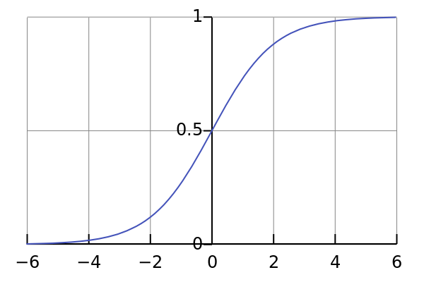
In the output f is the value of $\eta$ on the link scale. These are tiny values, most of the action in the logit (== logistic) function happens between -4 and 4:

(Image from Wikipedia: https://en.wikipedia.org/wiki/Logistic_function)

So we need to recentre the values of our linear predictor around say 0. The -5 in gratia::sim_binary() is doing this for the function you can simulate from in gratia.

`sim_binary2` <- function(x, scale = 5, shift = 5, ...) {
    ilink <- inv_link(binomial())
    x <- (x - shift) * scale
    p <- ilink(x)
    tibble(y = rbinom(n = p, size = 1, prob = p), f = x)
}

# the known linear predictor
lp <- x1 + x2 + f1_x1*fac1 + f2_x1*fac2 + f1_x2*fac1 + f2_x2*fac2 + 
     ((f1_x1*f1_x2) * fac1) + ((f2_x1*f2_x2) * fac2)

# simulate binary data
yb <- sim_binary2(lp, scale = scale, shift = -15)

After a bit of trial and error I used a value of -15 for the shift.

Now we can fit our model:

m_bin <- gam(y ~ fte(x1, x2, by = fac),
         method = "REML", data = yb, family = binomial())

but we now also get a warning:

> m_bin <- gam(y ~ te(x1, x2, by = fac), 
             method = "REML", data = yb, family = binomial())                   
Warning message:
In newton(lsp = lsp, X = G$X, y = G$y, Eb = G$Eb, UrS = G$UrS, L = G$L,  :
  Fitting terminated with step failure - check results carefully
> summary(m_bin)                                                              

Family: binomial 
Link function: logit 

Formula:
y ~ fac + te(x1, x2, by = fac)

Parametric coefficients:
             Estimate Std. Error z value Pr(>|z|)
(Intercept)    -151.6   623644.4       0        1
fac2            982.6  5116057.1       0        1

Approximate significance of smooth terms:
                 edf Ref.df Chi.sq p-value
te(x1,x2):fac1 3.981   4.05      0       1
te(x1,x2):fac2 3.000   3.00      0       1

R-sq.(adj) =      1   Deviance explained =  100%
-REML = -123.35  Scale est. = 1         n = 100

wherein the problem is immediately clear: we can perfectly predict the data, the massive standard errors on the parametric terms are an indicator of (quasi) complete separation. I haven't had time yet to look into why, but I suspect it is the values of the functions you are using the two groups. I think they are just too different on the link scale so it is trivial to guess the 0s and 1s once you know the fac.

Something to think about; you don't actually include any group means in your linear predictor (simulated data). The only differences between the groups comes in the form of the values 3 and 2 used in the exponential functions.