On the cradle of the Elo Rating System, and how to find it

Question

A definitive proposal can be found in:

Elo, Arpad E. (August, 1967). The Proposed USCF Rating System, Its Development, Theory, and Applications. Chess Life XXII (8): 242-247.

How exactly are

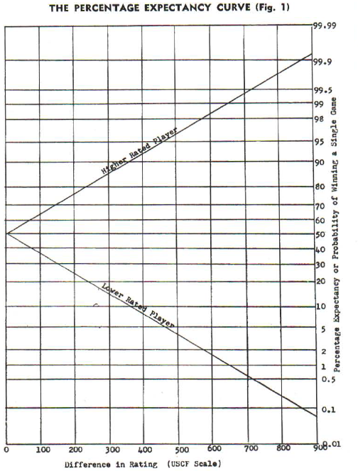
• THE PERCENTAGE EXPECTANCY CURVE (Fig. 1),
• TABLE I - RATING DIFFERENCES, and
• TABLE II- WINNING EXPECTANCIES

(page 243-244) calculated, including rounding details. I tried the normal distribution function with mean = 0 and sigma = 2000 / 7. But I could not get the rounding correct. For example the percentage expectancy of rating difference DP = 344 is 89% instead of 88% as in table II. Other irregularities: 54, 343, 358, 392, 620.

At page 247 we find a short reference list, including:

• A. E. Elo; Analytical Reports, 1961, 1963 & 1965; (Privately Printed).

Are these reports lost forever, or are copies preserved and available in the public domain?

Update

My question is not about the validity of the model, but about the calculation within the model. How exactly can I reproduce Table II? Why is the rating expectancy of DP = 344 equal to P = .88 instead of .89 as I would expect.

In The Rating of Chess players, Elo states in chapter 8.94 Development of the Percentage Expectancy Table:

For example, suppose D = 160. Then z = 160/284.84. The table gives .7143 and .2857. as the areas of the two portions under the curve. These probabilities are rounded to two figures in table 2.11.

Apparently Elo refers to a z-table, but which z-table was in use at that time (±1960)?

• @whuber I tried.

        σ=2000/7
  D   H |z-score |  Tabel (t)         |  t/2 + 50%      |  N(z)           | P
 54  58%| 0,189  |0.14990 71832 09998 |0,574953591604999|0,574953591604999| 57%

        | 1,200  |0.76986 06595 56583 |0,884930329778292|0,884930329778292|
 343 88%| 1,2005 |                    |  interpolatie   |0,885027364557095| 89%
        | 1,201  |0.77024 87986 71795 |0,885124399335897|0,885124399335898|

 344 88%| 1,204  |0.77141 04214 54696 |0,885705210727348|0,885705210727348| 89%
 358 90%| 1,253  |0.78979 42933 03286 |0,894897146651643|0,894897146651643| 89%
 392 92%| 1,372  |0.82993 65621 86873 |0,914968281093437|0,914968281093436| 91%
 620 99%| 2,170  |0.96999 31540 52536 |0,984996577026268|0,984996577026268| 98%

Source:

(Issued June 5, 1953). Tables of Normal Probability Functions U. S. Applied Mathematics (23) (Department of Commerce National Bureau of Standards).

• @cdalitz, 2000/7 is folklore, used by the Dutch Chess federation. I have no reference from literature.

Constructing TABLE-1 from TABLE-2

Table I and II are effectively mirror-images. See also the FIDE Handbook B. Permanent Commissions / 02. FIDE Rating Regulations.

R-code

D <-
  c(  3,  10,  17,  25,  32,  39,  46,  53,  61,  68,  76,  83,  91,  98, 106, 113, 121,
    129, 137, 145, 153, 162, 170, 179, 188, 197, 206, 215, 225, 235, 245, 256, 267, 278,
    290, 302, 315, 328, 344, 357, 374, 391, 411, 432, 456, 484, 517, 559, 619, 735, 736
   )

## TABLE I - RATING DIFFERENCES, between 51% and 99%.
## Column DP of TABLE-1 constitutes the midpoints of TABLE II, indexed by P.
## This is a reasonable approximation with the exception of P=99%.
table_1 <-
  head(cbind(P =seq(from=0.51, to=1.0, by=0.01),
             DP=trunc((head(D, -1) + tail(D, -1) + 1)/2) ),
       -1)
table_1

Constructing TABLE II - WINNING EXPECTANCIES with sigma = 200 * (10/7)

Note (10/7) is a rough approximation of sqrt(2). Conversion of rating difference to z-score gives at most 4 significant digits, which is useful when using a table indexed by z-score.

## Create rating differences, winning expectancy between 1 and 736, from 50% upto 100%.
n     <- 736
Pfull <- rep(-1, n)
pct   <- 0.50
k     <- 1
for(i in seq_along(D) ){
  while(k <= D[i]){
    Pfull[k] <- pct
    k        <- k + 1
  }
  pct <- pct + 0.01
}

## calculate / add normal probabilities (pnorm).
# P2, P15 probabilities rounded by 2, 15 digits.
df <- data.frame(D=seq(n), P=Pfull)

Deviations in Elo's expectations table

sd <- 200 * (10/7)  # standard deviation, using (10/7) instead of sqrt(2).
within(df,
{ P15 =  round(pnorm(D / sd , 0, 1,1), 15)
  P2  = round(P15, 2)
  attP2  = round(P - P2,  10)
}
) -> df2
subset(df2, attP2 != 0)

      D    P attP2   P2       P15
54   54 0.58  0.01 0.57 0.5749536
343 343 0.88 -0.01 0.89 0.8850274
344 344 0.88 -0.01 0.89 0.8857052
358 358 0.90  0.01 0.89 0.8948971
392 392 0.92  0.01 0.91 0.9149683
620 620 0.99  0.01 0.98 0.9849966

Constructing TABLE II by interpolation, third try

Consider rating values in steps of 20. The corresponding Z-score step is 20 * 7 / 2000 = 0.07. Finding the percentage scores corresponding to the rating values D = 0, 20, 40, etc. does not require any calculations. They can be extracted directly from the Z-table.

To calculate the intermediate values, linear interpolation is the most obvious. For example calculate the P value of 54 as follows:

sd  = 2000 / 7, the standard deviation chosen to ensure discrete steps in the Z table.
D   = 40 + 14, where 14 is the index in rating range 40-60
Z_b = 40 * 7 / 2000 = 0.14,  P_b = 0.5557 (From the Z table)
Z_e = Z_b + 0.07    = 0.21   P_e = 0.5832 (From the Z table)

The step size of P becomes: (0.5832 - 0.5557) / 20 = 0.001375

This gives:

P4  =  0.5557 + 14 * 0.001375 = 0.57495
    = 0.57495 + 5E-5 + 1E-6, rounded up to two decimals gives
P42 = 58%.

R-code.

dD <- 20                                          # step in D = 0, 20, 40, etc.
sd <- 2000 / 7                                    # standard deviation.
dZ <- dD / sd                                     # Short table, Z in two decimals.
within(df,
{ Z_sc    <- D / sd                               # 4 decimals.
  P15     <- round(pnorm(Z_sc), 15)               # value from extended table (1953).       
  Z_b     <- trunc(D / dD) * dD * 7 / 2000        # index in short table, begin.
  Z_e     <- Z_b + dZ                             # index in short table, end.
  P_b     <- round(pnorm(Z_b ), 4)                # P before.
  P_e     <- round(pnorm(Z_b + dZ), 4)            # P after.

  ##  Corrections to fit Elo tables.
  ## P_b[340:359] <- .8830 - .0010                  # Feller = .8836 
  ## P_b[380:399] <- .9082 + .0001                  # Feller = .9083 

  ix      <- D %% dD                              # index 0 - 20.
  Pstep   <- (P_e - P_b) / dD                     # interpolation step.

  ## Pstep[340:359] <- Pstep[320:339]               # Previous step size
  ## Pstep[380:399] <- Pstep[380:399] + .00001      # .00545 --> .00555

  P4e     <- P_b + ix * Pstep                     # intermediate percentage.
  P42e    <- round(P4e + 5E-5 + 1E-6, 2)          # rounded up to next percentage.
  attP42e <- round(P42e - P, 15)                  # deviation .   
}
) -> inter_lin
#subset(inter_lin, D >= 340 & D <= 360)
subset(inter_lin, attP42e != 0)

Between D = 340 and D = 400 we find 4 deviations:

 D    P attP42e P42e     P4e   Pstep ix    P_e    P_b  Z_e  Z_b       P15   Z_sc
343 0.88    0.01 0.89 0.88498 0.00066  3 0.8962 0.8830 1.26 1.19 0.8850274 1.2005
344 0.88    0.01 0.89 0.88564 0.00066  4 0.8962 0.8830 1.26 1.19 0.8857052 1.2040
358 0.90   -0.01 0.89 0.89488 0.00066 18 0.8962 0.8830 1.26 1.19 0.8948971 1.2530
392 0.92   -0.01 0.91 0.91480 0.00055 12 0.9192 0.9082 1.40 1.33 0.9149683 1.3720

How did it happen? - It is easy to see that the table is not entirely consistent. Look at the number of rating differences assigned to a percentage:

  P  L  -  H   Range
.86 303 - 315   13 
.87 316 - 328   13 
.88 329 - 344   16 <<<
.89 345 - 357   13
.90 358 - 374   20

Since the expectation function is monotonically increasing, the difference between H and L should not decrease. The 16 is clearly an outlier.

The error in D = 392 can be explained by using .00555 instead of .00545 as the step size for the linear interpolation. Errors in D=343, 344, 358 can be explained by taking a wrong starting percentage (related to Z = 1.19), and the step size of the previous group.

The above is obvious an educated guess. I am afraid I have to visit the Royal Library in the Hague to find out more.

Rounding - It is plausible that Elo confused the z boundary 1.2005 with 1.2050 (P=.885). That leaves D=54, D=358 to explain.

Now consider the folowing critical D values:

sigma = 200 * (10 / 7), z(D) = D / sigma.

  D  z(D)  P(D)  P-bndry  z-bndry   phi    plo   zlo  Truncated
 54 0.189 0.585 *  0.575 0.189231 0.5753 0.5714 0.18  Yes
 76 0.266 0.605    0.605 0.266316 0.6064 0.6026 0.26  No
106 0.371 0.645    0.645 0.371892 0.6480 0.6443 0.37  No
162 0.567 0.715    0.715 0.567941 0.7157 0.7123 0.56  No
188 0.658 0.745    0.745 0.658750 0.7454 0.7422 0.65  No
256 0.896 0.815    0.815 0.896538 0.8159 0.8133 0.89  No
358 1.253 0.905 *  0.895 1.253333 0.8962 0.8944 1.25  Yes

zpt = 0.189xxx is truncated to .189, so P-bndry( 54) is moved to the next bin.
zpt = 1.253xxx is truncated to .253, so P-bndry(358) is moved to the next bin.

However this logic is not applied to the other values.

Answer 1

I believe I have reverse engineered Arpa Elo's construction of Tables 1 and 2, irregularities included. Or at least I can posit a plausible explanation.

Like you I compared his Table 2 to a double precision calculation and found discrepancies at D = 54, 343, 344, 358, 392, and 620. I replicated your third try, performing linear interpolation between anchor points at D=0,20,40,... While having fun I also tried interpolating between D=0,1,2,... even though that would have been overly tedious for original hand calculation.

Thinking about how one would go about it with pen and paper, I believe what he did went like this. Find the 51 points on the z domain corresponding to the midpoints between p=0.50, 0.51, 0.05,...1.0. That is, the dividing lines are the z points that correspond to p=0.505, 0.515, 0.525... Convert integer D values to z using sigma=2000/7 as has been convincingly argued. Assign D to the nearest bin corresponding to p=0.50, 0.51... This provides Table 2, from which Table 1 is derived, as you point out.

This can be illustrated with the beginning entries.

row	z	p	p boundary	z boundary
1	0.00	0.5000
2	0.01	0.5040
interpolate			0.505	0.125
3	0.02	0.5080
4	0.03	0.5120
interpolate			0.515	0.0375
5	0.04	0.5160

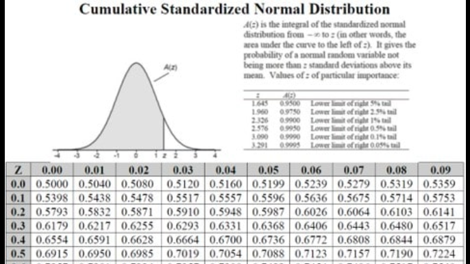
Where rounding in the code is implemented to match a (physical, paper) math handbook table, quantized to hundredths and taken out to 4 significant digits. Such as like this one, which I used when cross-checking.

The first dividing line is at p=0.505, a quarter of the way to row 3. With linear interpolation the corresponding value of z=0.0125. The second dividing line at p=0.515 corresponds to z=0.0375.

Then run through the range of D.

D	z	thresholding	bin assignment	p assignment
0	0.0	z < 0.0125	50	0.50
1	0.0035	z < 0.0125	50	0.50
2	0.007	z < 0.0125	50	0.50
3	0.0105	z < 0.0125	50	0.50
4	0.014	0.0125 <= z < 0.0375	51	0.51

Continue out to D=800.

Now about the irregularities. It seems that Elo made three clerical errors in his hand calculations, involving the dropping or mis-transcribing of a single digit. These mistakes look entirely plausible to me.

  Adjustments = {57: 0.1882, # correct is 0.1892 
                 88: 1.205,  # correct is 1.2005
                 89: 1.253}  # correct is 1.2533

When the the p/z decision boundaries are calculated in steps of 0.01 it comes out to the values in the table below. I have marked the three adjusted points with an asterisk.

p     z       p     z       p     z       p     z       p     z   
----- ------  ----- ------  ----- ------  ----- ------  ----- ------    
0.505 0.0125  0.515 0.0375  0.525 0.0627  0.535 0.0877  0.545 0.1130  
0.555 0.1383  0.565 0.1636  0.575 0.1882* 0.585 0.2146  0.595 0.2405  
0.605 0.2663  0.615 0.2924  0.625 0.3187  0.635 0.3451  0.645 0.3719  
0.655 0.3989  0.665 0.4261  0.675 0.4539  0.685 0.4817  0.695 0.5100  
0.705 0.5389  0.715 0.5679  0.725 0.5979  0.735 0.6279  0.745 0.6588  
0.755 0.6903  0.765 0.7226  0.775 0.7553  0.785 0.7893  0.795 0.8239  
0.805 0.8596  0.815 0.8965  0.825 0.9346  0.835 0.9740  0.845 1.0152  
0.855 1.0583  0.865 1.1032  0.875 1.1505  0.885 1.2050* 0.895 1.2530* 
0.905 1.3106  0.915 1.3720  0.925 1.4393  0.935 1.5142  0.945 1.5982  
0.955 1.6956  0.965 1.8114  0.975 1.9600  0.985 2.1700  0.995 2.5750  

To illustrate, apply this to D=54, the first irregularity. D=54 jumps bins on account of its z value, 0.189, being compared to a lower boundary of 0.1882 instead of the correct to four decimal places 0.1892.

D	z	thresholding	bin assignment	p assignment
53	0.1855	0.1636 <= z < 0.1882	57	0.57
54	0.189	0.1882 <= z < 0.2146	58	0.58
55	0.1925	0.1882 <= z < 0.2146	58	0.58
56	0.196	0.1882 <= z < 0.2146	58	0.58

Not being a statistician I have never programmed in R, but I hope example python code is useful. This program contains some extra bulk to print out Elo's two tables.

#!/usr/bin/python3
#----------------
import os,sys
import math
import numpy as np
import scipy

def lookup_cumm_norm(x, precision=4):
  # precision=4 simulates a physical handbook lookup table
  return round(scipy.stats.norm.cdf(x), precision)

# ---------------------------------------------------------------------------------------
def convert_binning_to_tables(p2d_bucket):
  """
  Returns:
  d2p: create mapping table d -> p, with p already quantized
       to hundredths above. Add in negative d by symmetry. 
  p2d: create mapping table p -> d (single midpoint value).
  """
  d2p = {}
  p2d = {}

  for bin in sorted(p2d_bucket.keys()):
    perc = round(bin / 100.0, 2)
    beg = p2d_bucket[bin][0]
    end = p2d_bucket[bin][-1]
    mid = math.floor((beg + end) / 2)
    if bin == 50: mid = 0
    if bin == 100: mid = 800

    for d in range(beg, end+1): 
      d2p[-d] = round(1 - perc, 2)
      d2p[d] = perc

    psym = round(1 - perc, 2)
    p2d[psym] = -mid
    p2d[perc] = mid

  # p2d_bucket is tacked on for convenience
  return d2p, p2d, p2d_bucket

# ---------------------------------------------------------------------------------------
def calc_fide_ratings_conversion_tables():

  sigma = 200 * 10 / 7 
  inv_sigma = 1 / sigma

  print("Sigma: 200*10/7 =", sigma)
  print("invSigma: 7/2000 =", inv_sigma)
  print("Algorithm: 1. place 51 dividing lines in z-domain located where p=0.505, 0.515...")
  print("              linearly interpolating between adjacent standard norm table entries")
  print("           2. apply 3 adjustments to account for clerical errors of hand construction") 
  print("           3. convert D in range [0,800] to z, assign z to nearest bin below threshold")
  print("           4. build Elo's Table 2 by mapping p=[0.0, 0.01.., 1.0] to ranges of D")
  print("           5. derive Table 1 from Table 2, mapping p onto the midpoint of D ranges\n")

  Adjustments = {57: 0.1882, # correct is 0.1892
                 88: 1.205,  # correct is 1.2005
                 89: 1.253}  # correct is 1.2533

  # Step 1. locate the decision lines on the z-axis of the cummulative normal function 
  bin = 50
  tgt = round(bin/100.0 + 0.005, 3)
  decision_lines = []
  
  for z in np.arange(0.0, 3.01, 0.01):
    plo = lookup_cumm_norm(z)
    phi = lookup_cumm_norm(z + 0.01)
    
    if plo == tgt:
      decision_lines.append((bin, z))
      bin += 1
      tgt = round(bin/100.0 + 0.005, 3)

    elif plo < tgt and tgt < phi:
      if bin in Adjustments:
        zpt = Adjustments[bin]
      else:
        stride = (tgt - plo) / (phi - plo)
        zpt = round(z + 0.01 * stride, 4)

      decision_lines.append((bin, zpt))
      bin += 1
      tgt = round(bin/100.0 + 0.005, 3)

  decision_lines.append((bin, z))

  # Step 2. place every rating difference value D from 0..800 into integer bins 50..100
  bucket = {}
  for bin in range(50,101):
    bucket[bin] = []

  # for every integer D in [0,800] convert D to its z value
  # then find the nearest dividing line z for which p(D) < z
  # assign D to the corresponding integer bin in range [50,100]
  idx = 0  

  for D in range(0, 801):
    z = D * inv_sigma
    bin, dividing_line = decision_lines[idx]

    # the less-than test fits better than an <= test
    if z < dividing_line:
      bucket[bin].append(D)
    else:
      idx += 1
      bin, dividing_line = decision_lines[idx]
      bucket[bin].append(D)

  # Step 3.
  return convert_binning_to_tables(bucket)

# ---------------------------------------------------------------------------------------
def print_fide_rating_conversion_tables(d2p, p2d, p2d_bins):
  """
  dtp - rating delta d to performacne expectation probability p
  p2d - p in increments of 0.01 to midpoint rating difference d
  p2d_bins - maps p onto list a D values assigned to p
  """
  # print the FIDE 'p to dp' table
  line = '-' * 85
  print("8.1a The table of conversion from fractional score, p, into rating differences, dp.")
  print(line)
  print('|', end='')
  for bin in range(100, -2, -17):
    print('%6s|%6s' %('p ', 'dp  '), end='|')
  print()  
  print(line)

  for beg in range(100, 83, -1):
    print('|', end ='')
    for bin in range(beg, -2, -17):
      if bin >= 0:
        p = round(bin / 100.0, 2)
        d = p2d[p]
        print(' %.2f | %-4i' %(p, d), end =' |')
      else:
        print('%7s%7s' %('|','|'), end ='')
    print()
  print(line)

  # print the FIDE 'D to PD' table
  line = '-' * 89
  print("\n8.1b Table of conversion of difference in rating, D, into scoring probability PD.")
  print(line)
  print('|', end='')
  for bin in range(50, 100, 13):
    print('%8s | %-8s ' %('D  ', 'PD'), end=' |')
  print()
  print(line)
  print('|', end='')
  for bin in range(50, 100, 13):
    print('%8s | %-3s | %-3s' %('Rtg Dif', 'H', 'L'), end=' |')
  print()
  print(line)

  for beg in range(50, 63, 1):
    print('|', end ='')

    for bin in range(beg, 102, 13):
      if bin > 100:
        print('%10s %5s %5s' %('|','|','|'), end='')
      else:
        phi = round(bin / 100., 2)
        plo = round(1.0-phi, 2)
        slo = ('%.2f' %(plo)).lstrip('0')
        shi = ('%.2f' %(phi)).lstrip('0') if bin < 100 else '1.0'
        rlo = p2d_bins[bin][0]
        rhi = p2d_bins[bin][-1]
        if bin == 100:
          print(' %3s %-3i | %s | %s' %('>', rlo-1, shi, slo), end=' |')
        else:
          print(' %3i-%-3i | %s | %s' %(rlo, rhi, shi, slo), end=' |')
    print()
  print(line + '\n')

if __name__ == '__main__':
  tables = calc_fide_ratings_conversion_tables()
  print_fide_rating_conversion_tables(*tables)

The tables are titled 8.1a and 8.1b to match the FIDE handbook.

8.1a The table of conversion from fractional score, p, into rating differences, dp.
-------------------------------------------------------------------------------------
|    p |  dp  |    p |  dp  |    p |  dp  |    p |  dp  |    p |  dp  |    p |  dp  |
-------------------------------------------------------------------------------------
| 1.00 | 800  | 0.83 | 273  | 0.66 | 117  | 0.49 | -7   | 0.32 | -133 | 0.15 | -296 |
| 0.99 | 677  | 0.82 | 262  | 0.65 | 110  | 0.48 | -14  | 0.31 | -141 | 0.14 | -309 |
| 0.98 | 589  | 0.81 | 251  | 0.64 | 102  | 0.47 | -21  | 0.30 | -149 | 0.13 | -322 |
| 0.97 | 538  | 0.80 | 240  | 0.63 | 95   | 0.46 | -29  | 0.29 | -158 | 0.12 | -336 |
| 0.96 | 501  | 0.79 | 230  | 0.62 | 87   | 0.45 | -36  | 0.28 | -166 | 0.11 | -351 |
| 0.95 | 470  | 0.78 | 220  | 0.61 | 80   | 0.44 | -43  | 0.27 | -175 | 0.10 | -366 |
| 0.94 | 444  | 0.77 | 211  | 0.60 | 72   | 0.43 | -50  | 0.26 | -184 | 0.09 | -383 |
| 0.93 | 422  | 0.76 | 202  | 0.59 | 65   | 0.42 | -57  | 0.25 | -193 | 0.08 | -401 |
| 0.92 | 401  | 0.75 | 193  | 0.58 | 57   | 0.41 | -65  | 0.24 | -202 | 0.07 | -422 |
| 0.91 | 383  | 0.74 | 184  | 0.57 | 50   | 0.40 | -72  | 0.23 | -211 | 0.06 | -444 |
| 0.90 | 366  | 0.73 | 175  | 0.56 | 43   | 0.39 | -80  | 0.22 | -220 | 0.05 | -470 |
| 0.89 | 351  | 0.72 | 166  | 0.55 | 36   | 0.38 | -87  | 0.21 | -230 | 0.04 | -501 |
| 0.88 | 336  | 0.71 | 158  | 0.54 | 29   | 0.37 | -95  | 0.20 | -240 | 0.03 | -538 |
| 0.87 | 322  | 0.70 | 149  | 0.53 | 21   | 0.36 | -102 | 0.19 | -251 | 0.02 | -589 |
| 0.86 | 309  | 0.69 | 141  | 0.52 | 14   | 0.35 | -110 | 0.18 | -262 | 0.01 | -677 |
| 0.85 | 296  | 0.68 | 133  | 0.51 | 7    | 0.34 | -117 | 0.17 | -273 | 0.00 | -800 |
| 0.84 | 284  | 0.67 | 125  | 0.50 | 0    | 0.33 | -125 | 0.16 | -284 |      |      |
-------------------------------------------------------------------------------------

8.1b Table of conversion of difference in rating, D, into scoring probability PD.
-----------------------------------------------------------------------------------------
|     D   | PD        |     D   | PD        |     D   | PD        |     D   | PD        |
-----------------------------------------------------------------------------------------
| Rtg Dif | H   | L   | Rtg Dif | H   | L   | Rtg Dif | H   | L   | Rtg Dif | H   | L   |
-----------------------------------------------------------------------------------------
|   0-3   | .50 | .50 |  92-98  | .63 | .37 | 198-206 | .76 | .24 | 345-357 | .89 | .11 |
|   4-10  | .51 | .49 |  99-106 | .64 | .36 | 207-215 | .77 | .23 | 358-374 | .90 | .10 |
|  11-17  | .52 | .48 | 107-113 | .65 | .35 | 216-225 | .78 | .22 | 375-391 | .91 | .09 |
|  18-25  | .53 | .47 | 114-121 | .66 | .34 | 226-235 | .79 | .21 | 392-411 | .92 | .08 |
|  26-32  | .54 | .46 | 122-129 | .67 | .33 | 236-245 | .80 | .20 | 412-432 | .93 | .07 |
|  33-39  | .55 | .45 | 130-137 | .68 | .32 | 246-256 | .81 | .19 | 433-456 | .94 | .06 |
|  40-46  | .56 | .44 | 138-145 | .69 | .31 | 257-267 | .82 | .18 | 457-484 | .95 | .05 |
|  47-53  | .57 | .43 | 146-153 | .70 | .30 | 268-278 | .83 | .17 | 485-517 | .96 | .04 |
|  54-61  | .58 | .42 | 154-162 | .71 | .29 | 279-290 | .84 | .16 | 518-559 | .97 | .03 |
|  62-68  | .59 | .41 | 163-170 | .72 | .28 | 291-302 | .85 | .15 | 560-619 | .98 | .02 |
|  69-76  | .60 | .40 | 171-179 | .73 | .27 | 303-315 | .86 | .14 | 620-735 | .99 | .01 |
|  77-83  | .61 | .39 | 180-188 | .74 | .26 | 316-328 | .87 | .13 |   > 735 | 1.0 | .00 |
|  84-91  | .62 | .38 | 189-197 | .75 | .25 | 329-344 | .88 | .12 |         |     |     |
-----------------------------------------------------------------------------------------

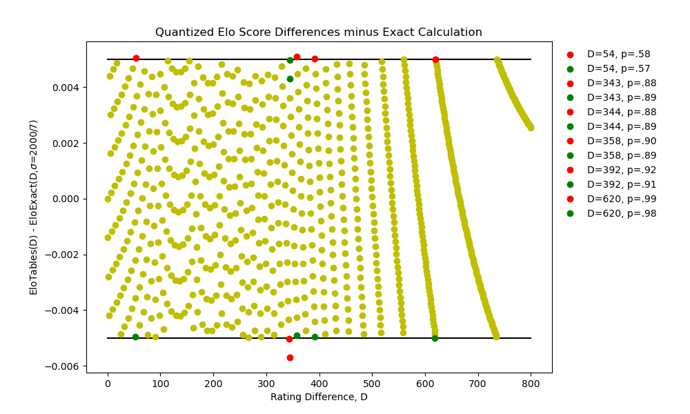
Addendum 1: Adding a visualization of score differences between Elo/FIDE tables and an exact calculation. Red dots are the mistakes in the official tables. Green dots show the corresponding corrected locations.

Addendum 2: Although not strictly on the topic of how to reproduce Elo's ratings conversion tables (without using a photocopier!), it's worth mentioning that his Table I contains inaccuracies as well. This is because the D(P) values of Table I are derived from Table II by extracting the midpoint of the corresponding "Rtg Dif" entries, truncated downward in the case of non-integer midpoints. Instead, correct is to find the nearest neighbor value of D. The inaccuracies are at most a single integer though, except for the upper reaches of p=0.98 and p=0.99. This table shows where I find deviations.

 p     dp    d     dp-d 
-----  ----- ----- -----
 0.51  7     7    
 0.52  14    14   
 0.53  21    22    -1
 0.54  29    29   
 0.55  36    36   
 0.56  43    43   
 0.57  50    50   
 0.58  57    58    -1
 0.59  65    65   
 0.60  72    72   
 0.61  80    80   
 0.62  87    87   
 0.63  95    95   
 0.64  102   102  
 0.65  110   110  
 0.66  117   118   -1
 0.67  125   126   -1
 0.68  133   134   -1
 0.69  141   142   -1
 0.70  149   150   -1
 0.71  158   158  
 0.72  166   167   -1
 0.73  175   175  
 0.74  184   184  
 0.75  193   193  
 0.76  202   202  
 0.77  211   211  
 0.78  220   221   -1
 0.79  230   230  
 0.80  240   240  
 0.81  251   251  
 0.82  262   262  
 0.83  273   273  
 0.84  284   284  
 0.85  296   296  
 0.86  309   309  
 0.87  322   322  
 0.88  336   336  
 0.89  351   350    1
 0.90  366   366  
 0.91  383   383  
 0.92  401   401  
 0.93  422   422  
 0.94  444   444  
 0.95  470   470  
 0.96  501   500    1
 0.97  538   537    1
 0.98  589   587    2
 0.99  677   665   12
 1.00  *     800  

Column dp is the official table value. d is the nearest neighbor integer. (In his August 1967 Chess Life magazine article, "* indicates an indeterminate value".)

Update 1: recalculation with more precise Cumulative Standard Normal Distribution table

As mentioned in the comments Elo likely made recourse to tables with a precision of 0.001, in contrast to above where I simulated tables in z steps of 0.01. Recomputation of Table 2 supports this suggestion. Performing the calculations without any injected adjustments reduces the number of discrepancies by one. Previously the list is D = [54, 343, 344, 358]. Now the list is D = [343, 344, 358].

This listing compares the computed z-boundary values under the two assumptions. Below, "hit" indicates a direct table lookup of the sought p-boundary value.

               z-step = 0.01     | z-step = 0.001
               -------------     | ----------------
 bin  p-bndry    bracket z-bndry | z-bndry  bracket      | z-6digit  z-diff
----  -------    ------- ------- | -------  -------      | --------  ------
  50    0.505  0.01-0.02  0.0125 |  0.0125  0.012-0.013  | 0.012533 -0.0000
  51    0.515  0.03-0.04  0.0375 |  0.0375  0.037-0.038  | 0.037608 -0.0001
  52    0.525  0.06-0.07  0.0627 |  0.0628  0.062-0.063  | 0.062707  0.0001
  53    0.535  0.08-0.09  0.0877 |  0.0878  0.087-0.088  | 0.087845 -0.0000
  54    0.545  0.11-0.12  0.1130 |  0.1130  hit          | 0.113039 -0.0000
  55    0.555  0.13-0.14  0.1383 |  0.1383  0.138-0.139  | 0.138304 -0.0000
  56    0.565  0.16-0.17  0.1636 |  0.1637  0.163-0.164  | 0.163658  0.0000
  57    0.575  0.18-0.19  0.1892 |  0.1890  hit          | 0.189118 -0.0001
  58    0.585  0.21-0.22  0.2146 |  0.2148  0.214-0.215  | 0.214702  0.0001
  59    0.595  0.24-0.25  0.2405 |  0.2405  0.240-0.241  | 0.240426  0.0001
  60    0.605  0.26-0.27  0.2663 |  0.2662  0.266-0.267  | 0.266311 -0.0001
  61    0.615  0.29-0.30  0.2924 |  0.2923  0.292-0.293  | 0.292375 -0.0001
  62    0.625  0.31-0.32  0.3187 |  0.3187  0.318-0.319  | 0.318639  0.0001
  63    0.635  0.34-0.35  0.3451 |  0.3450  hit          | 0.345126 -0.0001
  64    0.645  0.37-0.38  0.3719 |  0.3717  0.371-0.372  | 0.371856 -0.0002
  65    0.655  0.39-0.40  0.3989 |  0.3988  0.398-0.399  | 0.398855 -0.0001
  66    0.665  0.42-0.43  0.4261 |  0.4262  0.426-0.427  | 0.426148  0.0001
  67    0.675  0.45-0.46  0.4539 |  0.4538  0.453-0.454  | 0.453762  0.0000
  68    0.685  0.48-0.49  0.4817 |  0.4818  0.481-0.482  | 0.481727  0.0001
  69    0.695        hit  0.5100 |  0.5100  hit          | 0.510073 -0.0001
  70    0.705  0.53-0.54  0.5389 |  0.5388  0.538-0.539  | 0.538836 -0.0000
  71    0.715  0.56-0.57  0.5679 |  0.5680  hit          | 0.568051 -0.0001
  72    0.725  0.59-0.60  0.5979 |  0.5978  0.597-0.598  | 0.597760  0.0000
  73    0.735  0.62-0.63  0.6279 |  0.6280  hit          | 0.628006 -0.0000
  74    0.745  0.65-0.66  0.6588 |  0.6588  0.658-0.659  | 0.658838 -0.0000
  75    0.755  0.69-0.70  0.6903 |  0.6903  0.690-0.691  | 0.690309 -0.0000
  76    0.765  0.72-0.73  0.7226 |  0.7223  0.722-0.723  | 0.722479 -0.0002
  77    0.775  0.75-0.76  0.7553 |  0.7553  0.755-0.756  | 0.755415 -0.0001
  78    0.785  0.78-0.79  0.7893 |  0.7893  0.789-0.790  | 0.789192  0.0001
  79    0.795  0.82-0.83  0.8239 |  0.8240  hit          | 0.823894  0.0001
  80    0.805  0.85-0.86  0.8596 |  0.8597  0.859-0.860  | 0.859617  0.0001
  81    0.815  0.89-0.90  0.8965 |  0.8965  0.896-0.897  | 0.896473  0.0000
  82    0.825  0.93-0.94  0.9346 |  0.9347  0.934-0.935  | 0.934589  0.0001
  83    0.835  0.97-0.98  0.9740 |  0.9740  hit          | 0.974114 -0.0001
  84    0.845  1.01-1.02  1.0152 |  1.0153  1.015-1.016  | 1.015222  0.0001
  85    0.855  1.05-1.06  1.0583 |  1.0580  hit          | 1.058122 -0.0001
  86    0.865  1.10-1.11  1.1032 |  1.1030  hit          | 1.103063 -0.0001
  87    0.875  1.15-1.16  1.1505 |  1.1505  1.150-1.151  | 1.150349  0.0002
  88    0.885  1.20-1.21  1.2005 |  1.2005  1.200-1.201  | 1.200359  0.0001
  89    0.895  1.25-1.26  1.2533 |  1.2535  1.253-1.254  | 1.253565 -0.0001
  90    0.905  1.31-1.32  1.3106 |  1.3105  1.310-1.311  | 1.310579 -0.0001
  91    0.915  1.37-1.38  1.3720 |  1.3720  hit          | 1.372204 -0.0002
  92    0.925  1.43-1.44  1.4393 |  1.4395  1.439-1.440  | 1.439531 -0.0000
  93    0.935  1.51-1.52  1.5142 |  1.5140  hit          | 1.514102 -0.0001
  94    0.945  1.59-1.60  1.5982 |  1.5980  hit          | 1.598193 -0.0002
  95    0.955  1.69-1.70  1.6956 |  1.6950  hit          | 1.695398 -0.0004
  96    0.965  1.81-1.82  1.8114 |  1.8120  hit          | 1.811911  0.0001
  97    0.975        hit  1.9600 |  1.9600  hit          | 1.959964  0.0000
  98    0.985        hit  2.1700 |  2.1690  hit          | 2.170090 -0.0011
  99    0.995  2.57-2.58  2.5750 |  2.5730  hit          | 2.575829 -0.0028

With regards to bin=57 the z-boundary in the updated calculation has shifted from 0.1892 to 0.189. This places D=54 right on the dividing line. By the less-than-or-equals test on the lower boundary D=54 is assigned to the p=0.58 bin, as is found in Elo's Table 2.

D	z	thresholding	bin assignment	p assignment
53	0.1855	0.1637 <= z < 0.1882	57	0.57
54	0.189	0.189 <= z < 0.2146	58	0.58
55	0.1925	0.189 <= z < 0.2146	58	0.58
56	0.196	0.189 <= z < 0.2148	58	0.58

For D=343, 344, and 358 an adjustment is still required to accommodate presumed clerical errors. For bin=88 and bin=89 there is little change to the z-boundary values. Only two corrections now need to be assumed. Using the same adjustments as before serves to generate the official tables.

  Adjustments = {88: 1.205,  # correct is 1.2005 from linear interp using tables with 0.001 z-step
                 89: 1.253}  # correct is 1.2535 ...

Running through the values for bin 89 I find that any z-value in the range [1.2496 - 1.2530] removes the discrepancy of D=358. Rounding up to 1.254 does not. A figure of 1.253 seems to me to be the most plausible mistake of transcription or calculation, so I encode that value.

Answer 2

There is a book by Elo entirely devoted to his formulas:

Arpad. E. Elo: "The Rating of Chessplayers." Ishi Press, 1978

Although the book presents some formulas, the derivation is not argued in details, and some formulas only hold under strong (rarely holding) assumptions, and it is not even discussed what these assumptions are or whether the estimators are biased or consistent. Just as one example, consider the "performance rating formula" (1) in your cited article. It can be derived by the "method of moments", i.e. by equating an expected value with its observed value as follows:

1. If a player of unknown rating $r$ plays against $n$ players with ratings $q_1,\ldots,q_n$, then the expected number of wins $W$ is $$E(W) = \sum_{j=1}^n \Phi(r-q_j)$$ where $\Phi$ is the normal distribution function with mean zero and variance $\sigma^2$.
2. Setting the observed number of wins $\hat{W}$ equal to the expected number of wins in the above formula yields an equation for $r$, that cannot be solved in closed form.
3. For solving this equation, Elo makes the assumption (without even mentioning it) that $\sum_j \Phi(x_i) = \Phi\left(\sum_i x_i\right)$ and obtains $$\Phi^{-1}\left(\frac{\hat{W}}{n}\right) + \frac{1}{n} \sum_j q_j = r$$ which is the "performance rating formula" (1).
4. Obviously, Elo's assumption does not hold unless $\Phi$ is a linear function, and at some later point (p. 133, equation(18) in the 1978 book above) he says that $\Phi(x)$ may be taken as $x/4\sigma$ "for the most used portion of the curve". Unfortunately, he did not explain how he arrived at this approximation. A Taylor expansion of $\Phi$ around $x=0$ would yield $\Phi(x)\approx x/\sqrt{2\pi}\sigma $, and $\sqrt{2\pi}$ is considerably different from 4, so it is not clear how Elo derived his approximation. Fortunately, this (presumable) error does not matter much, because he later subsumes the factor $4\sigma$ together with other factors in a value $K$, for which he suggests two different choices, depending on the number $n$ of played games. In any case, the linear approximation only holds when the ratings of all players are quite close to each other.

For a more lucid presentation of the mathematical model and an accurate derivation of estimation formulas (which are different from Elo's formulas), see

Batchelder, William H., and Neil J. Bershad. "The statistical analysis of a Thurstonian model for rating chess players." Journal of Mathematical Psychology 19.1 (1979): 39-60.

The discussed model differs from Elo's model, though, in the additional assumption that a chess game can result in ties (Elo only uses a model with two possible outcomes: win or loss, and draws are later counted in the formulas as half wins, which means that you cannot compute the probability of a draw with Elo's model). Elo's model can be obtained, however, as a special case of Batchelder's and Bershad's model simply by assuming that a tie is impossible and thereby setting the "tie width" $t$ to zero.

To address your question what the three terms mean in the context of the model, we must frst define the model: $$P(\mbox{i wins against j})=\Phi(r_i - r_j)$$ where $\Phi$ is the distribution function of the normal (or alternatively: logistic) distribution with zero mean and standard deviation $\sigma$. In the cited article Elo alleges that he uses $\sigma=200$, but this does not match the tables listed in his article. Table I should be $\Phi^{-1}$ and Table II $\Phi$. I obtain approximately similar numbers with the choice $\sigma=286$, e.g.

> # reproduce values from Table I
> qnorm(0.60, sd=286)
[1] 72.45727
> qnorm(0.19, sd=286)
[1] -251.0783

or

> # reproduce values from Table II
> pnorm(210, sd=286)
[1] 0.7686066
> pnorm(95, sd=286)
[1] 0.6301187

which approximately matches the numbers in the tables. The alleged choice of $\sigma=200$ is also inconsistent with the use of a logistic distribution:

> plogis(220, s=200*sqrt(3)/pi)
[1] 0.88029

which is very far from the number given by Elo.

Answer 3

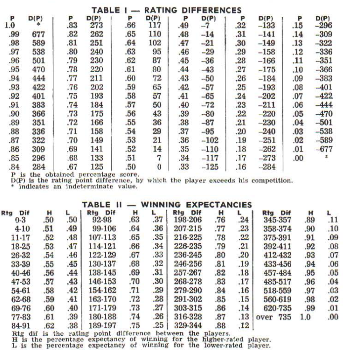
Below we see the specific tables from Elo, Arpad E. (August, 1967). The Proposed USCF Rating System, Its Development, Theory, and Applications. Chess Life XXII (8): 242-247.

The values in table I seem to be an average of the values in table II (rather than a direct computation with the quantile function).

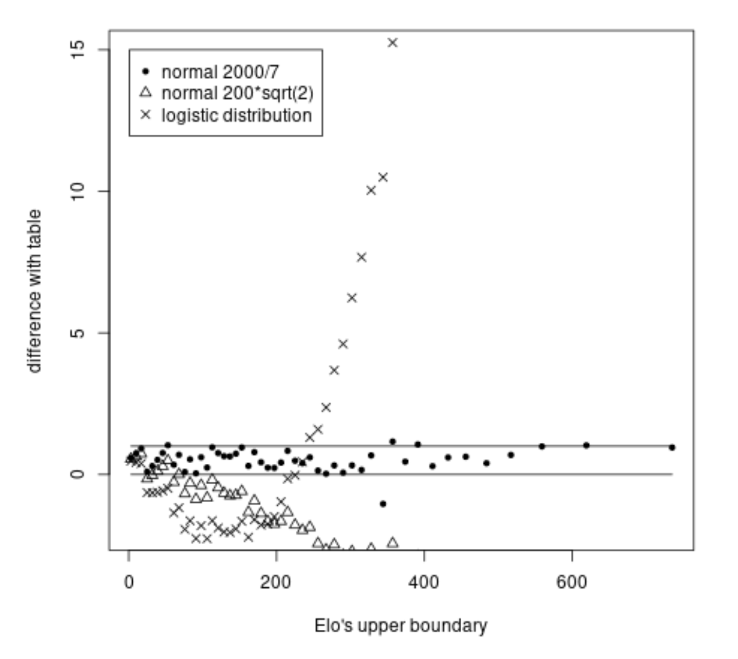
The values in table II correspond very well with a normal distribution that has standard deviation $2000/7$. The upper boundaries will be equal to the percentile scores of the normal distribution rounded down and the lower boundaries will be equal to the percentile scores of the normal distribution rounded up. Below you see a comparison of three methods.

The logistic distribution or a normal distribution with standard deviation $200 \sqrt{2}$ have large differences.

For the normal distribution with standard deviation $2000/7$ there are some small discrepancies, but only of the order of $\pm 1$ and that can be due to round-off errors and use of tables with lower precision* or possibly a typo.

p = seq(0.505,0.995,0.01)
elo1 = qnorm(p,0,2000/7)
elo2 = qnorm(p,0,200*sqrt(2))
elo3 = -log10(1/p-1)*400

x = c(3,10,17,25,32,39,46,53,61,68,76,83,91,98,106,113,121,129,137,145,153,162,170,179,188,197,206,215,225,235,245,256,267,278,290,302,315,328,344,357,374,391,411,432,456,484,517,559,619,735)

plot(x,x-x, type = "l", xlab = "Elo's upper boundary", log = "", ylim = c(-2,15), ylab = "difference with table")
points(x,elo1-x, pch = 20)
points(x,elo2-x, pch = 2)
points(x,elo3-x, pch = 4)

legend(1,15, c("normal 2000/7", "normal 200*sqrt(2)", "logistic distribution"), cex = 1, pch = c(20,2,4))

lines(x,x*0+1)

---

In 'The rating of chess players, past and present' Elo writes an example

For example. let D = 160. Then z = 160/282.84 = .566. The table gives .7143 and .2857 as the areas of the two portions under the curve. These probabilities are rounded to two figures in table 2.11

This suggests that he used sufficiently accurate tables with at least 4 figures. An example could be Table X (copied from Pearson) in Garrett's 'statistics in psychology and education' which occurs as a reference.

Answer 4

Elo was specific: "This basic relationship ... turns out to be the familiar cumulative proportion curve of probability theory, the 'standard sigmoid'." That's an old-fashioned way of saying that differences on the rating scale are linearly related to Z-scores: standard Normal deviates.

Here is his plot of that relationship for differences of scores, which therefore are nominally $200\sqrt{2}\approx 283$ per standard deviation unit:

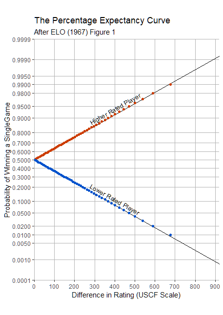
This evidently is hand drawn. Here is my plot of the same, but using a scale of $202.3\sqrt{2}$ because that matches the tables better:

The dots plot the values from Table 1. The entire point is that on this Normal probability plotting scale, the relationship between ratings and probability is linear.

Plotting the difference between the rating difference "$d(P)$" and the rating as computed from the Normal distribution from the probability "$P$" (the residuals in the foregoing plot) suggests Elo used an approximation that works poorly in the tails (beyond the central 95% of the distribution, more or less). (More detailed study suggests this is a severely truncated rational approximation.) The worst discrepancy is at the end, where the score difference of 677 really should be 666.

Those who want details might be interested in the code that generated this figure.

#
# Table 1.
#
d <- c(677, 589, 538, 501, 470, 444, 422, 401, 383, 366, 351, 336, 322, 309, 296, 284,
       273, 262, 251, 240, 230, 220, 211, 202, 193, 184, 175, 166, 158, 149, 141, 133, 125,
       117, 110, 102, 95, 87, 80, 72, 65, 57, 50, 43, 36, 29, 21, 14, 7, 0)
p <- seq(1.0, 0.50, length = length(d) + 1)[-1]
X <- data.frame(P = p, Delta = d)
#
# The transformations relating "P" to "d(P)" in the table.
#
F. <- function(x, lambda = 202.3 * sqrt(2)) pnorm(x / lambda)
Q. <- function(p, lambda = 202.3 * sqrt(2)) lambda * qnorm(p)
X$Q <- round(Q.(X$P), 0)
X$Check <- with(X, Delta - Q)
with(X, plot(Delta, round(Q.(P) / Delta - 1, 3)))
with(X, plot(Delta, Q.(P) - Delta))
X$F <- round(F.(X$Delta), 3)
with(X, plot(P, round(F.(Delta) - P, 3)))
#
# Replot Figure 1.
#
y <- c(.01, .1, .5, 1, 2, 5, 10, 20, 30, 40)
y <- c(y, 50, 100 - rev(y)) / 100                        # The y grid
x <- seq(0, 900, by = 100)                               # The x grid

library(ggplot2)
X <- subset(X, P < 1)
scale.USCF <- 202.3
rho <- 4/3 * diff(range(x)) / diff(range(qnorm(y)))      # 4/3 is aspect ratio
alpha <- atan(rho / scale.USCF * sqrt(2) / 2) * 180 / pi # Angles of the lines

ggplot(data.frame(x = x)) +
  geom_vline(aes(xintercept = x), col = gray(0.7)) +
  geom_hline(aes(yintercept = y), data = data.frame(y = y), col = gray(0.7)) +
  geom_abline(slope = c(-1, 1) * 1 / (scale.USCF * sqrt(2))) +
  geom_point(aes(Delta, P), data = X, col = hsv(0.05, 1, .8)) + 
  geom_point(aes(Delta, 1 - P), data = X, col = hsv(.6, 1, .8)) + 
  coord_fixed(ylim = range(y), xlim = c(0, 920), expand = FALSE, ratio = rho) +
  scale_y_continuous(trans = scales:::probability_trans("norm"), breaks = y) +
  scale_x_continuous(breaks = x) + 
  annotate("text", x = rep(400, 2), y = pnorm(c(1.58, 0.36 - 1.58)),
           label = paste(c("Higher", "Lower"), "Rated Player"),
           angle = alpha * c(1, -1), size = 3.5) +
  xlab("Difference in Rating (USCF Scale)") +
  ylab("Probability of Winning a SingleGame") +
  ggtitle("The Percentage Expectancy Curve", "After ELO (1967) Figure 1") + 
  theme(panel.grid = element_blank(),
        panel.background = element_blank())