Discrete-time survival model output doesn't match Cox proportional-hazards model - problem with input of data?

Question

I'm trying to construct a discrete-time survival model to analyse some mating data. I've used a Cox proportional hazards model previously but got some input that the discrete-time survival model would fit my data better.

The previous post and my results I got from R there can be found here and can work as a good background for understanding my output.

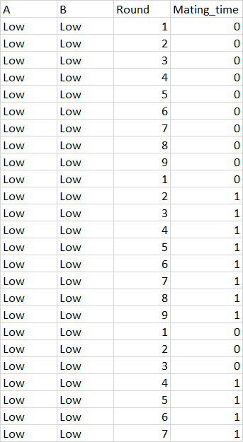
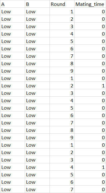
When I tried to do the discrete-time survival model I didn't even get close to the results I got from the Cox proportional hazards model. I've reformatted my data to the following format:

and the list goes on..

I have three different combinations of A and B that is:

A           B
High        High
Low         Low
Metabolite  Metabolite

I'm interested in comparing when mating occurs between the different treatment (observation round 1-9 - in my dataset called Round) and if mating occur Mating_time = 1 during that round and if mating time didn't occur = 0. I also wan to look at the interaction between A and B (A*B)

I've fitted the data to a glm in the following manner:

mod<-glm(Round ~ Mating_time + A*B,data=dat, family = "binomial")

and then when running ANOVA I get the following output:

> Anova(mod)
Analysis of Deviance Table (Type II tests)

Response: Round
                LR Chisq Df Pr(>Chisq)
Mating_time      0.46970  1     0.4931
A                0.00027  2     0.9999
B                0.00024  2     0.9999
A : B            0.00041  4     1.0000

This is completely different from my previous result posted here (same link as before)

I'm wondering if anyone have a clue what I've done wrong. Should the data instead be coded as 1 for Mating_time for all the observations after mating have occurred?

E.g.

EDIT:

I've now edited the raw data table as suggested below and fixed the mistake with mating_time and round. The script looks like this:

mod<-glm(Mating_time ~ Round + A*B,data=dat, family = "binomial")

Anova(mod)

and the output is:

> Anova(mod)
Analysis of Deviance Table (Type II tests)

Response: Mating_time
                LR Chisq Df Pr(>Chisq)    
Round             35.005  8  2.668e-05 ***
A                  3.925  2    0.14048    
B                  8.912  2    0.01161 *  
A : B             10.314  4    0.03545 *  
---
Signif. codes:  0 ‘***’ 0.001 ‘**’ 0.01 ‘*’ 0.05 ‘.’ 0.1 ‘ ’ 1

I understand that "Round" is important in the model, but when running post-hoc test. If I'm simply interested in AB interaction, and not Round+AB, could I simply do emmeans as follows:

multcomp::cld(emmeans(mod, ~A|B), Letters = letters, reversed = T) # Post-Hoc test

If I run:

multcomp::cld(emmeans(mod, ~Mating_round+A|B), Letters = letters, reversed = T) # Post-Hoc test

I get a very messy table with the "Round" also incorporated. Although its important to fit it into the original model.

The output of:

   multcomp::cld(emmeans(mod, ~A|B), Letters = letters, reversed = T) # Post-Hoc test

looks the following:

> multcomp::cld(emmeans(mod, ~A|B), Letters = letters, reversed = T) # Post-Hoc test
F1_diet = Metabolite:
 F0_diet     emmean    SE    df   asymp.LCL asymp.UCL .group
 Normal       -1.77   0.239 Inf     -2.24     -1.30     a    
 Metabolite   -1.91   0.209 Inf     -2.32     -1.50     a    
 Low          -1.91   0.235 Inf     -2.37     -1.45     a    

F1_diet = Normal:
 F0_diet     emmean    SE    df asymp.LCL asymp.UCL  .group
 Low          -1.34   0.242 Inf     -1.82     -0.87     a    
 Normal       -2.29   0.265 Inf     -2.81     -1.77     b   
 Metabolite   -2.55   0.277 Inf     -3.09     -2.00     b   

F1_diet = Low:
 F0_diet     emmean    SE   df  asymp.LCL asymp.UCL .group
 Normal       -2.22   0.247 Inf     -2.70     -1.73     a    
 Low          -2.50   0.278 Inf     -3.05     -1.96     a    
 Metabolite   -2.58   0.247 Inf     -3.07     -2.10     a    

Results are averaged over the levels of: Round 
Results are given on the logit (not the response) scale. 
Confidence level used: 0.95 
Results are given on the log odds ratio (not the response) scale. 
P value adjustment: tukey method for comparing a family of 3 estimates 
significance level used: alpha = 0.05 
NOTE: If two or more means share the same grouping symbol,
      then we cannot show them to be different.
      But we also did not show them to be the same. 

The particular line "Results are averaged over the levels of: Round" in the emmeans output means that the rounds are covered in the post-hoc test right?

EDIT

I've made suggested edits and data str() looks like this:

> str(mod)
tibble [1,549 × 4] (S3: tbl_df/tbl/data.frame)
 $ A           : chr [1:1549] "Low" "Low" "Low" "Low" ...
 $ B           : chr [1:1549] "Low" "Low" "Low" "Low" ...
 $ Round       : Factor w/ 9 levels "1","2","3","4",..: 1 2 3 4 5 6 7 8 9 1 ...
 $ Mating_time : num [1:1549] 0 0 0 0 0 0 0 0 0 0 ...

Although I still get output in Anova (as for the response of the df =1):

> Anova(mod)
Analysis of Deviance Table (Type II tests)

Response: Mating_time
                        LR Chisq Df Pr(>Chisq)    
as.factor(Round       )   35.094  8  2.571e-05 ***
A                          3.749  2    0.15343    
B                          9.024  2    0.01097 *  
A : B                     10.424  4    0.03385 *  
---
Signif. codes:  0 ‘***’ 0.001 ‘**’ 0.01 ‘*’ 0.05 ‘.’ 0.1 ‘ ’ 1

and post-hoc test (now with all 9 comparisons, still just post it for df question) :

> multcomp::cld(emmeans(mod, ~A*B), Letters = letters, reversed = T) # Post-Hoc test
   A           B        emmean  SE  df asymp.LCL asymp.UCL .group
 Low        Normal       -1.49 0.213 Inf     -1.91     -1.08  a    
 Normal     Metabolite   -1.87 0.218 Inf     -2.29     -1.44  ab   
 Metabolite Metabolite   -1.98 0.192 Inf     -2.35     -1.60  ab   
 Low        Metabolite   -1.99 0.217 Inf     -2.42     -1.57  ab   
 Normal     Low          -2.26 0.230 Inf     -2.71     -1.81  ab   
 Normal     Normal       -2.35 0.249 Inf     -2.84     -1.86  ab   
 Low        Low          -2.55 0.265 Inf     -3.07     -2.03   b   
 Metabolite Normal       -2.59 0.264 Inf     -3.10     -2.07   b   
 Metabolite Low          -2.62 0.236 Inf     -3.09     -2.16   b   

Results are averaged over the levels of: Round 
Results are given on the cloglog (not the response) scale. 
Confidence level used: 0.95 
Note: contrasts are still on the cloglog scale 
P value adjustment: tukey method for comparing a family of 9 estimates 
significance level used: alpha = 0.05 
NOTE: If two or more means share the same grouping symbol,
      then we cannot show them to be different.
      But we also did not show them to be the same. 

Related to the comment by EdM about the degrees of freedom: There's no change in degrees of freedom from the changes I've made for Round being a factor, I've also had Mating_time and Round as a factor but didn't change the output of the df.

Answer 1

As your intent was to set up a binary regression that would be similar to a Cox survival model, you evidently treated the time variable Round as a factor instead of as a numeric predictor, even though the values of Round were numbers. As a Cox model makes no assumptions about the functional form of the baseline hazard, a corresponding binomial regression should treat Round as a factor rather than a numeric predictor so that there is no assumption about the functional form of its association with log-odds of mating.

There would be nothing inherently wrong about treating Round as a numeric predictor. The danger, however, is that is easy to do inadvertently when the time-period values are numbers. Unless you specify otherwise, the software might then interpret the time variable as a numeric predictor linearly related to the log-odds of an event.

If you do want to treat the time variable as numeric in a discrete-time model, a strict linear association with log-odds of an event would be unrealistic. A flexible fit, for example with a regression spline or other type of generalized additive model for the time variable, would be better.

If I want to model a numeric time value as a factor, I find it safest to state that explicitly, as in:

modFactor <- glm(Mating_time ~ as.factor(Round) + A*B, data=dat, family = "binomial")

That provides separate coefficient estimates for log-odds differences of each of the Round values from the first. The associations of A, B and their interaction with the log-odds of mating are modeled as the same regardless of the value of Round, around the baseline log-odds for each Round. Note that you aren't restricted to the default "logit" link for the binomial regression; a "cloglog" link is more closely related to a Cox survival model.

Once the model is built, in post-modeling analysis you can evaluate both the overall significance of the model and illustrate the differences among specific scenarios.

The significant A:B interaction coefficient by itself already indicates that the association of each of A and B with outcome depends on the value of the other, at least in some combinations. With 3 levels of each of A and B, however, it doesn't tell you which particular combinations differ from each other.

The additional displays produced by emmeans() provide ways to document those differences, in ways that you choose. The way that you chose for your first example displays the estimates of the log-odds of mating, averaged over all values of Round, comparing the 3 levels of F0_diet within each of the 3 values of F1_diet, and makes multiple-comparison corrections only within each value of F1_diet. Depending on the question you are asking that could be OK, but a combined evaluation of all 9 diet combinations at once might be expected by a reviewer. That's what you added in a later version of the question.

In your model there is no interaction between Round and the other predictors. Thus the associations of A, B and their interaction with outcome in the log-odds scale of outcomes will be the same regardless of Round. If you are working in that scale, you thus could choose any particular Round as an example to illustrate the A:B interaction, rather than using the averages over all values of Round. The different baseline log-odds for the different values of Round, however, would mean different associations of A, B, and their interaction with outcomes in the probability scale depending on the Round.