Understanding a beta-variational autoencoder

Question

I'm working on a beta-variational autoencoder using car images from the Vehicle Color Recognition Dataset. At this point, I'm just exploring different architectures and values for beta. (If you're interested, the notebook is here, but it is very much a work in progress, a bit sloppy at this point, and will certainly be changing as I explore beta-VAEs.)

Here is an example of some generated images with an encoding layers of size 16, 3 convolutional layers, and a beta values of 1e-5, 1e-3, and 1e-1.

And another set with encoding size 256, 3 convolutional layers, and the same values for beta.

In both cases, starting at the third row, it looks like posterior mode collapse and the resulting model is not capturing any details. These images appear more like an overall average of all images. Does this make sense?

The second row looks like more reasonable images, albeit quite blurry and not quite the quality I was hoping for. Any suggestions on how to improve these images?

Row 1 is a complete mystery to me. While the images are certainly car-like, they are very cartoony or hallucinogenic. Any ideas what is going on here?

I appreciate any comments and suggestions.

Answer 1

After a couple of weeks of digging into my VAE, I think I have an understanding of what I'm seeing. Referring to the images from the original question...

• In the first row, KL divergence has a very low weight. Looking at the learned mean and standard deviation values, I find that the distribution of means is fairly wide, ranging in values from around -5 to 5. For standard deviation, the distribution is extremely wide with values of -100 to 100, or higher. The KL divergence cost should drive the distributions of mean and standard deviations to be centered on 0 and 1, resp., and presumably not have a huge variability. My hypothesis is that the effective lack of KL divergence penalty is leading to a VAE that is behaving lake a standard AE. Images are mapped to points int he latent space, but the space is not necessarily smooth. When images are generated from random points in the latent space, the results are these garbled images.

• The second row has an intermediate weight for KL divergence and the generated images are much more reasonable. Looking at the learned distributions of means and standard deviations, the are very well centered on 0 and 1 and have low variance. This represents an ideal situation with a balanced penalty for reconstruction and KL divergence.

• For the third row, KL divergence has a high weight, and the distributions are again very well centered on 0 and 1 but have extremely low variance. When random samples are drawn from these distributions, the values are nearly always zero or very close to zero. My interpretation is that these are the "average" vehicle. I tested generating images with purely zeros for latent space values and the generated images are identical to those in the third row.

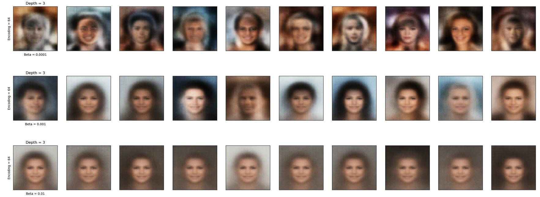
I explored this with another dataset, the CelebA Attributes dataset with images of celebrity faces, and saw very similar results. In the figure, below, the first row has low weighted KL divergence, the second row has a medium weight, and the third row has a high way. As I saw with the vehicles images, low weight images are garbled, medium weight images are reasonable, and high weight images all look the same and are the same as images from all zero inputs (the average face image).