Approximating the distribution of the product of iid beta variates

Question

Background

I am interested in the distribution of

$$\theta_0=1-\prod_{i=1}^n(1-\theta_i)$$

where the $\theta_{i>0}$ are iid beta random variates:

$$\theta_{i>0}\sim\text{Beta}(\alpha,\beta)$$

In my case $\beta\gg1\gg\alpha$ and $n\gg1$, so I used the following transformation:

$$\phi_i=-\ln(1-\theta_i)\\\theta_i=1-e^{-\phi_i}\\d\theta_i=e^{-\phi_i}\\p(\phi_i)\propto(1-e^{-\phi_{i}})^{\alpha-1}e^{-\phi_{i}\beta}\qquad\text{(1)}$$

With $\beta\gg\alpha$, $\theta_i$ and $\phi_i$ tend to be very small, so

$$1-e^{-\phi_i}\approx\phi_i$$

Substituting into (1) gives:

$$p(\phi_i)\hspace{1mm}\dot\propto\hspace{1mm}\phi_i^{\alpha-1}e^{-\phi_i\beta}$$

Or

$$\phi_i\hspace{1mm}\dot\sim\hspace{1mm}\text{Gamma}(\alpha,\beta)$$

Define $\phi_0$:

$$\phi_0\equiv\sum_{i=1}^n\phi_i$$

Using the properties of the gamma distribution:

$$\phi_0\hspace{1mm}\dot\sim\hspace{1mm}\text{Gamma}(n\alpha,\beta)$$

Finally,

$$\theta_0=1-e^{-\phi_0}$$

(I can further improve the approximation through moment matching to get slightly different values of $\alpha$ and $\beta$ to use in the gamma distribution, but this doesn't affect the question below.)

Question

What would be a good way to quantifiably demonstrate how well the above approximation works for varying values of $\alpha$, $\beta$, and $n$?

For a single set of values, I can use simulation, e.g.,

set.seed(214462480)
alpha <- 2e-3
beta <- 1001
n <- 1e3
theta0.sim1 <- -expm1(replicate(1e5, sum(log1p(-rbeta(n, alpha, beta)))))
theta0.sim2 <- -expm1(-rgamma(1e5, n*alpha, beta))
ks.test(theta0.sim1, theta0.sim2)$p.value
#> [1] 0.5396774

And the ecdf lines are right on top of each other.

However, simulation in this manner is slow and defeats the purpose of the approximation. $\alpha$ and $\beta$ are sampled from a joint posterior, so I require a large number of samples of $\theta_0$, each with varying $\alpha$ and $\beta$ parameters. Furthermore, this will be applied to a number of problems, so $n$ and the distributions of $\alpha$ and $\beta$ can also vary.

Answer 1

This is just an extended comment. One can obtain the exact distribution (and mean and variance) of $\phi_{i>0}$ although for the values of $\alpha$ and $\beta$ you mention, the result differs little from your approximation. (It can make a big difference for other values of $\alpha$ and $\beta$.)

Again, using Mathematica:

dist = TransformedDistribution[-Log[θ], θ \[Distributed] BetaDistribution[β, α]];

PDF[dist, ϕ]

μϕ = Mean[dist]
(* -PolyGamma[0, β] + PolyGamma[0, α + β] *)

σ2ϕ = Variance[dist]
(* PolyGamma[1, β] - PolyGamma[1, α + β] *)

sol = Solve[{μϕ == a b, σ2ϕ == a b^2}, {a, b}][[1]]

For your values of $\alpha=2/1000$ and $\beta=1001$ the values of $a$ and $b$ are

sol /. {β -> 1001, α -> 2/1000} // N
{a -> 0.002, b -> 0.000999499}

Answer 2

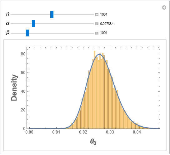
Here is a "visual" approach (using Mathematica) to check on the gamma approximation for the distribution of $\theta_0$.

nsamples = 10000; (* Number of random samples *)
Manipulate[
 (* Random sample of θ0 values *)
 x = RandomVariate[BetaDistribution[β, α], {nsamples, n}];
 θ0 = 1 - Times @@ # & /@ x;
 
 (* Find gamma distribution parameters with same mean and variance *)
 (* θ0Var = E(θi^2)^n - E(θi)^(2n) *);
 θ0Var = (Variance[BetaDistribution[β, α]] + Mean[BetaDistribution[β, α]]^2 // Together)^n -
   Mean[BetaDistribution[β, α]]^(2 n);
 θ0Mean = 1 - Mean[BetaDistribution[β, α]]^n;
 {a, b} = {a0, b0} /. Solve[{θ0Mean == a0 b0, θ0Var == a0 b0^2}, {a0, b0}][[1]] // Quiet;
 
 (* Display histogram and approximating gamma density *)
 Show[Histogram[θ0, "FreedmanDiaconis", "PDF", PlotRange -> {{0, Automatic}, Automatic},
   Frame -> True, FrameLabel -> (Style[#, Bold, 18] &) /@ {"\!\(\*SubscriptBox[\(θ\), \(0\)]\)",  "Density"}],
  Plot[PDF[GammaDistribution[a, b], z], {z, 0, 1}, PlotRange -> All, PlotPoints -> 100]],
 {{n, 1001, Style["n", Italic, 14]}, 10, 2000, 1, Appearance -> "Labeled"},
 {{α, 1/1000, Style["α", 14]}, 1/1000, 1/10, Appearance -> "Labeled"},
 {{β, 1001, Style["β", 14]}, 50, 5000, Appearance -> "Labeled"}
 ]

Something similar could be done with a cdf.

The values of $a$ and $b$ for the approximating gamma distribution are

$$a=\frac{\left(\left(\frac{\beta }{\alpha +\beta }\right)^n-1\right)^2}{\left(\frac{\beta ^2+\beta }{(\alpha +\beta ) (\alpha +\beta +1)}\right)^n-\left(\frac{\beta }{\alpha +\beta }\right)^{2 n}}$$

$$b=\frac{\left(\frac{\beta }{\alpha +\beta }\right)^{2 n}-\left(\frac{\beta ^2+\beta }{(\alpha +\beta ) (\alpha +\beta +1)}\right)^n}{\left(\frac{\beta }{\alpha +\beta }\right)^n-1}$$

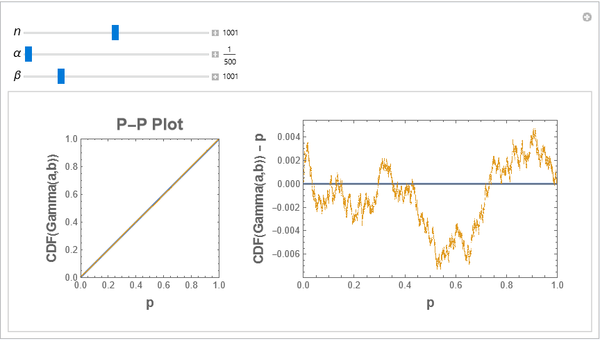
The above code can be modified to produce a P-P plot (as suggested by @whuber):

nsamples = 10000; (* Number of random samples *)
Manipulate[
 (* Random sample of θ0 values *)
 x = RandomVariate[BetaDistribution[β, α], {nsamples, n}];
 θ0 = 1 - Times @@ # & /@ x // Sort;
 
 (* Find gamma distribution parameters with same mean and variance *)
 (* θ0Var = E(θi^2)^n - E(θi)^(2n) *);
 θ0Var = (Variance[BetaDistribution[β, α]] + Mean[BetaDistribution[β, α]]^2 // Together)^n -
   Mean[BetaDistribution[β, α]]^(2 n);
 θ0Mean = 1 - Mean[BetaDistribution[β, α]]^n;
 {a, b} = {a0, b0} /. Solve[{θ0Mean == a0 b0, θ0Var == a0 b0^2}, {a0, b0}][[1]] // Quiet;
 
 (* Display histogram and approximating gamma density *)
 t = Table[{i/nsamples, CDF[GammaDistribution[a, b], θ0[[i]]], 
    CDF[GammaDistribution[a, b], θ0[[i]]] - (i - 1/2)/nsamples},
   {i, nsamples}];
 GraphicsRow[{ListPlot[{{{0, 0}, {1, 1}}, t[[All, {1, 2}]]}, 
    Joined -> {True, False}, Frame -> True, 
    PlotRange -> {{0, 1}, {0, 1}}, AspectRatio -> 1,
    PlotLabel -> Style["P-P Plot", Bold, 18], 
    FrameLabel -> (Style[#, Bold, 14] &) /@ {"p", "CDF(Gamma(a,b))"}],
   ListPlot[{{{0, 0}, {1, 0}}, t[[All, {1, 3}]]}, 
    Joined -> {True, False}, Frame -> True, PlotRange -> {{0, 1}, Automatic},
    FrameLabel -> (Style[#, Bold, 14] &) /@ {"p", "CDF(Gamma(a,b)) - p"}]}],

 {{n, 1001, Style["n", Italic, 14]}, 10, 2000, 1, Appearance -> "Labeled"},
 {{α, 2/1000, Style["α", 14]}, 1/1000, 1/10, Appearance -> "Labeled"},
 {{β, 1001, Style["β", 14]}, 50, 5000, Appearance -> "Labeled"},
 TrackedSymbols :> {n, α, β}]

The plot on the right highlights the size of the departures for a particular random sample.