Frobenius norm of a product of Gaussian matrices

Question

Suppose $$C_n=X_1 X_2\cdots X_n,$$ where $X_i$ is $d\times d$ matrix with IID entries normally distributed with mean 0 and variance $\frac{1}{d}$.

The following appears to be true for large $d$, why?

$$\|C_n C_n^T\|_F^2\approx d(n+1).$$

Here are some numbers from 4 samples with $d=1000$ (Notebook):

n     sample1  sample2  sample3  sample4
----------------------------------------
1     2003.99  1998.66  1999.51  1998.14
2     3029.97  2990.12  3008.21  2999.13
3     3967.81  3995.46  4022.33  4005.20
4     5027.41  5075.39  4941.94  5057.40
5     6143.21  5964.35  5844.76  6015.08

Answer 1

Let $X$ be $d\times d$ a random matrix with iid $\mathcal N(0, 1/d)$ elements. Let us first show that $$\| XX^\top \|^2 \approx 2d.$$

Induction base

We want to compute expectations of squared elements of $\sum_j X_{ij}X_{kj}$.

Consider diagonal elements first: those are $\sum_j X_{ij} X_{ij} = \sum_j X_{ij}^2$. In this sum each term has expectation $1/d$ and there are $d$ of them, so the sum has expectation $1$. The variance is $O(1/d)$, so we can ignore it. Then the expectation of the square is approximately $1^2 = 1$, and there are $d$ of them, contributing $d$ to the squared norm.

Now off-diagonal elements: those are $\sum_j X_{ij}X_{kj}$. Each term has mean 0 and variance $1/d^2$ (product of $1/d$ and $1/d$), after summation we have mean 0 and variance $1/d$. After squaring, we get expected value $1/d$. There are $(d^2-d)$ off-diagonal elements, which is approximately $d^2$, so in total this contributes approximately $d$ to the squared norm.

Together, we get $2d$.

Induction step

Now we need to show that if $A$ has diagonal elements with mean $1$ and off-diagonal elements with variance $k/d$, then $XA X^\top$ will have diagonal elements with mean $1$ and off-diagonal variance approximately $(k+1)d$. It will then follow that $$\| XA X^\top \|^2 \approx d + (k+1)d.$$

In coordinates, $XA X^\top$ is $\sum_{jk} X_{ij} A_{jk} X_{lk}$. Again, considering diagonal elements first, we should look at $j=k$ terms, which are $\sum_j X_{ij}^2 A_{jj}$. Each term has expectation $1/d$, we have $d$ of them, so the total expected value is 1. The variance can be ignored. Done.

Now off-diagonal elements. We want their variance, which is the same as the expectation of their squares. The squares are: $$\big(\sum_{jk} X_{ij} A_{jk} X_{lk}\big)\cdot \big(\sum_{ab} X_{ia} A_{ab} X_{lb}\big) = \sum_{jkab} X_{ij} A_{jk} X_{lk} X_{ia} A_{ab} X_{lb}.$$ We only need terms that have non-zero expectation. There are two kinds of terms like that:

• if $j=a$ and $k=b$, then we get $X_{ij}^2 X_{lk}^2 A_{jk}^2$. This has expected value $1/d \cdot 1/d \cdot k/d = k/d^3$. And there are $(d^2-d)$ terms like that, which is approximately $d^2$ so we get expectation approximately $k/d$.
• if $j=a=k=b$, then we get $X_{ij}^2 X_{lj}^2 A_{jj}^2$. This has expected value $1/d \cdot 1/d \cdot 1 = 1/d^2$. And there are $d$ terms like that, so we get expectation $1/d$.

Together, the expectation is approximately $(k+1)/d$.

---

Code for sanity-checking:

import numpy as np
np.random.seed(42)

d = 1000
X = np.random.randn(d, d) / np.sqrt(d)

F = X @ X.T
print(f'Diagonal: {np.sum(np.diag(F)**2):.1f}\nTotal:    {np.sum(F**2):.1f}\n')

X = np.random.randn(d, d) / np.sqrt(d)
F = X @ F @ X.T
print(f'Diagonal: {np.sum(np.diag(F)**2):.1f}\nTotal:    {np.sum(F**2):.1f}')

Output:

Diagonal: 1002.8
Total:    2003.8

Diagonal: 1012.8
Total:    3029.2

Answer 2

Fix $n$, and let

$$ \Gamma = [d]^{n+1} = \{ \gamma = (\gamma_0, \gamma_1, \ldots, \gamma_n) : \gamma_i \in [d] \} $$

be the space of length-$n$ paths in $[d] = \{1, \ldots, d\}$. We also define

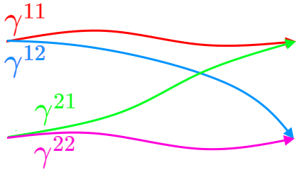
$$ \Gamma^{⧖} = \{ (\gamma^{11}, \gamma^{12}, \gamma^{21}, \gamma^{22}) \in \Gamma^4 : \gamma^{i1}_0 = \gamma^{i2}_0 \text{ and } \gamma^{1j}_n = \gamma^{2j}_n \}. $$

That is, $\Gamma^{⧖}$ is the space of all quadruples of curves $(\gamma^{11}, \gamma^{12}, \gamma^{21}, \gamma^{22})$ that form a configuration like below:

Then with $d\times d$ matrices $X^{(1)}, \ldots, X^{(n)}$ with IID $\mathcal{N}(0, d^{-1})$ entries and $C_n = X^{(1)} \cdots X^{(n)}$,

$$ \| C_n C_n^T \|_F^2 = \sum_{(\gamma^{11}, \gamma^{12}, \gamma^{21}, \gamma^{22}) \in \Gamma^{⧖}} \prod_{\substack{t \in [n] \\ i, j \in [2]}} X^{(t)}_{\gamma^{ij}_{t-1},\gamma^{ij}_t} $$

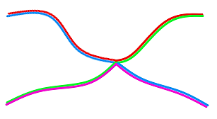
Expectation. We observe that, for the product $\prod_{t \in [n]; i, j \in [2]} X^{(t)}_{\gamma^{ij}_{t-1},\gamma^{ij}_t}$ to have non-zero expectation, each of the factor $X^{(t)}_{pq}$ must appear even number of times in the product. This forces the paths $\gamma^{11}, \gamma^{12}, \gamma^{21}, \gamma^{22}$ to coalesce. Among such coalesced configurations, the most abundant pattern is of the form

Since the "quadruple joint" in the above figure can occur at any of $t = 0, 1, \ldots, n$, the number of such configurations is $ (n+1) d^{n+1} (d-1)^n $, yielding

$$ \mathbf{E}[ \| C_n C_n^T \|_F^2 ] \sim (n+1) d^{n+1} (d-1)^n \cdot \mathbf{E}[(X_{pq}^{(t)})^2]^{2n} \sim (n+1)d. $$

---

Remark 1. Numerical simulation suggests that

$$ \mathbf{E}[ \| C_n C_n^T \|_F^2 ] = (n+1)d + \frac{n(n+1)}{2} + \mathcal{O}(d^{-1}) $$

as $d \to \infty$ for each $n$. When $n = 1, 2$, this claim can be directly verified by the exact formulas

$$ \mathbf{E}[ \| C_1 C_1^T \|_F^2 ] = 2d + 1, \qquad \mathbf{E}[ \| C_2 C_2^T \|_F^2 ] = 3d + 3 + \frac{3}{d}. $$

Remark 2. It seems that $\mathbf{Var}[ \| C_n C_n^T \|_F^2 ] = \mathcal{O}_n(1)$ as $d \to \infty$. For example, we have an exact formula

$$ \mathbf{Var}[ \| C_1 C_1^T \|_F^2 ] = 36 + \frac{40}{d} + \frac{20}{d^2}. $$

I will revisit this idea and try to (1) articulate more rigorous and detailed estimate of the expectation, and (2) prove the boundedness of the variance as $d \to \infty$. I'm just too exhausted and sleepy right now...