Distribution of a quantity similar to the $t$ statistic

Question

Suppose I have samples $A$ and $B$ from $N(\mu,\sigma^2)$ with unknown mean and variance. The sample sizes are $n_A$ and $n_B$. I construct two statistics: $$t_A=\frac{\bar X_A-\mu}{s_A/\sqrt{n_A}}$$ and $$t_{B/A}=\frac{\bar X_B-\mu}{s_A/\sqrt{n_A}}$$ where $\bar X$ is the sample mean $s$ is the sample standard deviation. Clearly, $t_A\sim t(n_A-1)$. I am interested in the distribution of $t_{B/A}$. Questions:

1. When $n_A=n_B=:n$, is it true that $t_{B/A}\sim t(n-1)$? I guess so because of the independence of sample mean and variance of a normal distribution.
2. When $n_A\neq n_B$, what is the distribution of $t_{B/A}$?

Answer 1

As to 1., yes, indeed, as we have an independent ratio of a standard normal and the square root of a chi-square root divided by its d.f. (for details, see below, setting $n_B=n_A$).

As to 2., we have by standard results that $$ \sqrt{n_B}(\bar{X}_B-\mu)/\sigma\sim N(0,1) $$ and $$ (n_A-1)\frac{s_A^2}{\sigma^2}\sim \chi^2_{n_A-1} $$ Write $$ \begin{eqnarray} t_{B/A}&=&\frac{\bar X_B-\mu}{s_A/\sqrt{n_A}}\\ &=&\frac{\sqrt{n_A}(\bar X_B-\mu)/\sigma}{\sqrt{\frac{s_A^2}{\sigma^2}}}\\ &=&\sqrt{\frac{n_A}{n_B}}\frac{\sqrt{n_B}(\bar X_B-\mu)/\sigma}{\sqrt{\frac{s_A^2}{\sigma^2}}}\\ \end{eqnarray} $$ Again, like in 1., $$ \frac{\sqrt{n_B}(\bar X_B-\mu)/\sigma}{\sqrt{\frac{s_A^2}{\sigma^2}}}\sim t(n_A-1), $$ so that $$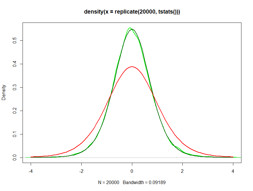t_{B/A}\sim \sqrt{\frac{n_A}{n_B}}t(n_A-1),$$ a scaled or non-standardized t-distribution with scale parameter $\sqrt{n_A/n_B}$, cf. https://en.wikipedia.org/wiki/Student%27s_t-distribution#Location-scale_t_distribution.

Illustration (reset nB <- nA if you want to illlustrate 1., also note the code allows for differing variances, see edit below):

library(extraDistr)
nA <- 10
nB <- 20

mu <- 0
sigmaA <- 2
sigmaB <- 2

tstats <- function(){
  A <- rnorm(nA, mu, sigmaA)
  B <- rnorm(nB, mu, sigmaB)

  tAB <- sqrt(nA)*mean(B)/sd(A)
}

plot(density(replicate(20000, tstats())), col="green", lwd=2, xlim=c(-4,4))
xax <- seq(-4, 4, by=0.1)
lines(xax, dlst(xax, df=nA-1, sigma=sqrt((sigmaB^2*nA)/(sigmaA^2*nB))), col="darkgreen", lwd=2)
lines(xax, dt(xax, df=nA-1), col="red", lwd=2)

EDIT in response to the comment below the question:

If the variances differ as in $Var(A_i)=\sigma_A^2$ and $Var(B_i)=\sigma_B^2$, we would write $$ \begin{eqnarray} t_{B/A}&=&\frac{\bar X_B-\mu}{s_A/\sqrt{n_A}}\\ &=&\sqrt{\frac{\sigma^2_B}{\sigma^2_A}}\frac{\sqrt{n_A}(\bar X_B-\mu)/\sigma_B}{\sqrt{\frac{s_A^2}{\sigma_A^2}}}\\ &=&\sqrt{\frac{\sigma^2_Bn_A}{\sigma^2_An_B}}\frac{\sqrt{n_B}(\bar X_B-\mu)/\sigma_B}{\sqrt{\frac{s_A^2}{\sigma_A^2}}}, \end{eqnarray} $$ again obtaining a scaled t with a different scaling factor.