Is lasso preferable to ridge or principal component regression in multicollinear settings?

Question

Consider a $N\times p$ data matrix $\mathbf X$ with columns $\mathbf x_j$. ESL recommends standardizing the inputs before performing ridge regression, which I understand to mean centering the columns $\mathbf x_j$ to have mean 0 and rescaling them to have variance $\|\mathbf x_j\|^2/N=1$. So let’s assume this is the case. I was thinking about the principle component directions in the column span $V\subset\mathbf R^N$ of $\mathbf X$ (a linear subspace of $\mathbf R^N$). These principal component directions $v\in\mathbf R^N$ have the property that they are norm-one vectors in $V$ so that the variance of $Xv$ is maximized (i.e. we want to maximize $\|Xv\|$).

Note that if I augment $\mathbf X$ by adding $n-1$ copies of $\mathbf x_p$ to the end (so that $\mathbf X$ is now $N\times(p+n-1)$), then the vector $v=(0,\ldots,0,1/\sqrt n,\ldots,1/\sqrt n)$ has norm 1, where there are $p-1$ zeros followed by $n$ entries with value $1/\sqrt n$.

Now $Xv=\frac{n}{\sqrt n}\mathbf x_p$ with norm $\sqrt{nN}$ and variance $(Xv\cdot Xv)/N=n$. Therefore for $n$ large enough, the projection of $v$ to $V$ will determine a principal component direction and some rescaling of $\mathbf x_p$ will be a principal component of $\mathbf X$.

Contrast this with the lasso, which, if we follow the modified least-angle regression algorithm, should be completely insensitive to the addition of the additional columns, since the LAR algorithm will analyze which column is best correlated with the residual at any given moment.

This is a completely artificial construction, but does it reflect a reason to prefer lasso to ridge regression in multi-collinear situations?

Answer 1

• Lasso vs Ridge, the difference between these two is whether you want to place more or less focus on parameter selection or on regularisation. Ridge will prefer more parameters but with more shrinking, Lasso will prefer fewer parameters but with less shrinking.

  See also: Why is LASSO considered good for selection but less good for reducing variance

  The characterisation of a multicollinearity setting is not so important here. The choice between these two will depend on your prior beliefs about the correct model. Are a large fraction of the variables important or only a small fraction. Do you want to remove the weeds (Lasso) or do you want to prune the branches (Ridge). Both can occur with or without multicollinearity.

• PCA will also reduce the model variability, but the philosophy is different. It is based on the idea that the regressor variables relate to some underlying structure like the PCA components. By using just those components you will reduce the model variability, but the motivation is the idea of capturing some underlying structure. If there is not such a structure, then PCA will have less effect (and, it might be opposite to the idea of Lasso which relates to the belief that a small selection of features are able to capture a model, with PCA you are blending all these features together).

Answer 2

I made some computational investigations into this issue and I concluded that perhaps it is actually a problem. Here is my Python code:

import numpy as np
import matplotlib.pyplot as plt
import math
p = 5
N = 7
rng = np.random.default_rng()
X = rng.random((N, p))
X = X - X.mean(axis=0)
X = X / X.std(axis=0)
def juice(j,t):
  Y = X
  for i in range(t):
    Y = np.append(Y,X[:,p-1].reshape(N,1), axis=1)
  U, D, Vh = np.linalg.svd(Y, full_matrices=False)
  pc1 = U[:,p-1]
  return np.linalg.norm(X[:,p-1]/np.linalg.norm(X[:,p-1])*np.sign(X[0,p-1])-U[:,j]*np.sign(U[0,j]))

data1 = np.array([[juice(j,i) for i in range(100)] for j in range(p)])
plt.plot(data1.T)
plt.show()

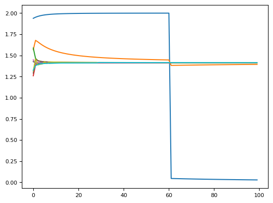
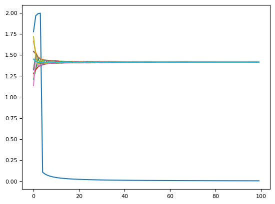
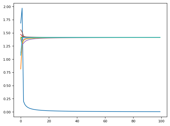
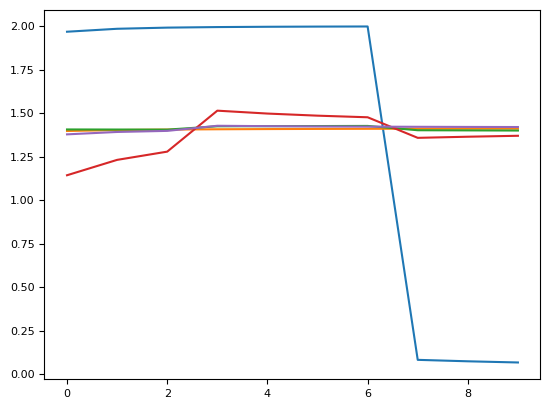
This code does the following: it generates an $N\times p$ matrix $X$ of numbers uniformly distributed on [0,1). Next, it standardizes the columns of $X$ to have mean 0 and variance 1. We then define a function which takes as inputs integers $j$ and $t$. The number $j$ will index which normalized principal component we’ll return (so $j=0$ returns the normalized first principal component). The counter $t$ determines how many copies of the last column we will append to the matrix $X$. Finally, we plot the norm of the difference between the last column of our original matrix $X$ (now normalized to have norm 1) and the $j$th normalized principal component of $X$, after correcting for possible sign flips.

I performed this with $p = 5$ and $N = 7$ as well as $p = 10$ and $N=70$. For $p=5$ and $N=7$ I produced this plot (the blue curve always corresponds to the $j=0$ first principal component):

For $p=10$ and $N=70$ I produced these plots:

So, in conclusion, it does seem possible to ‘overwhelm’ PCA with highly collinear datasets.