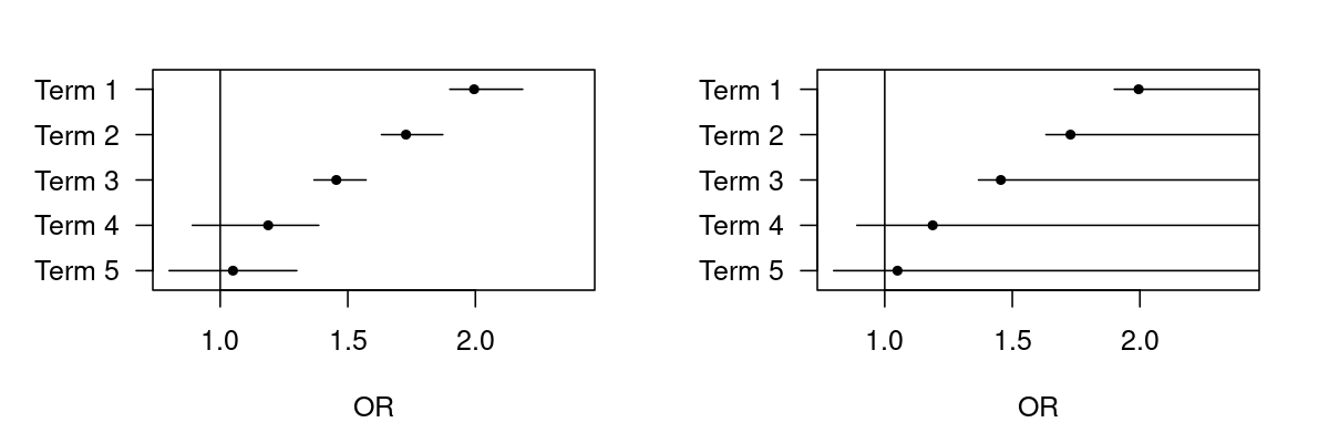
Many OR (odds ratio) visualizations show 95% confidence intervals expressing uncertainty like on the left panel in figure below.
However, in genomic overrepresentation analysis right tailed Fisher tests are used, fisher.test(., alternative='greater') on contingency tables such as,
      DE   nDE   Sum
IN    20    79    99
nIN 1869 13032 14901
Sum 1889 13111 15000
yielding infinite upper confidence bounds.
          OR  lower upper
Term_1 1.995 1.9000   Inf
Term_2 1.728 1.6320   Inf
Term_3 1.455 1.3677   Inf
Term_4 1.188 0.8910   Inf
Term_5 1.050 0.8000   Inf
Following this logic, a visualization should look like the one in the right panel, but I have never seen that.
Performing a two-sided test would yield a finite upper bound, which is not correct though.
I've heard we could use the confidence interval of a two-sided test with \alpha=0.1 in this case, but I'm not sure.
I considered bootstrapping the CIs, and tried it by perpetuating the p values of the differential gene expression matrix without replacement and use percentiles of the bootstrapped ORs, but this gave me upper bounds lower than the estimated OR. (I guess I can only bootstrap p values but not CIs.)
So how can appropriate confidence intervals or error margins be calculated, or uncertainty properly be expressed in visualization respectively?

