Distribution to describe size of population with random exponential growth

Question

Is there a distribution family that describes the size of a population experiencing random exponential growth (either discrete or continuous)?

For context, I am trying to computationally model a population of cells experiencing exponential growth. My modeling framework uses discrete timesteps, i.e. it evaluates whether a cell will divide after the passage of a short period of time dt. After each dt, each cell will divide with probability $r$ between 0 and 1.

This is my work so far:

Given some initial population size $n_0$ and $t = 0$, we will have population $n_1 = n_0 + [\textrm{# of cells from } n_0 \textrm{ that divided}]$ following a single timestep (let's say $t = 1$, i.e. dt = 1). The number of cells that divided is $\mathrm{Binom}(n_0, r)$, since it's a sum of $n_0$ $\mathrm{Bernoulli}(r)$ rvs, so $n_1 = n_0 + \mathrm{Binom}(n_0, r)$. The same would apply for $n_2$ and $n_3$ and so forth; in general, $n_k = n_{k-1} + \mathrm{Binom}(n_{k-1}, r)$ after $k$ timesteps.

I can't figure out if $n_k$ falls into any sort of known distribution. Expanded out, it looks like

$n_k = n_0 + \mathrm{Binom}(n_0, r) + \mathrm{Binom}(n_0 + \mathrm{Binom}(n_0, r), r) + \mathrm{Binom}(n_0 + \mathrm{Binom}(n_0, r) + \mathrm{Binom}(n_0 + \mathrm{Binom}(n_0, r), r), r) + \ldots$

a sum of binomial rvs, but each successive binomial has a size parameter dependent on the previous binomials. Is there a way to combine those binomials/simplify this at all?

Answer 1

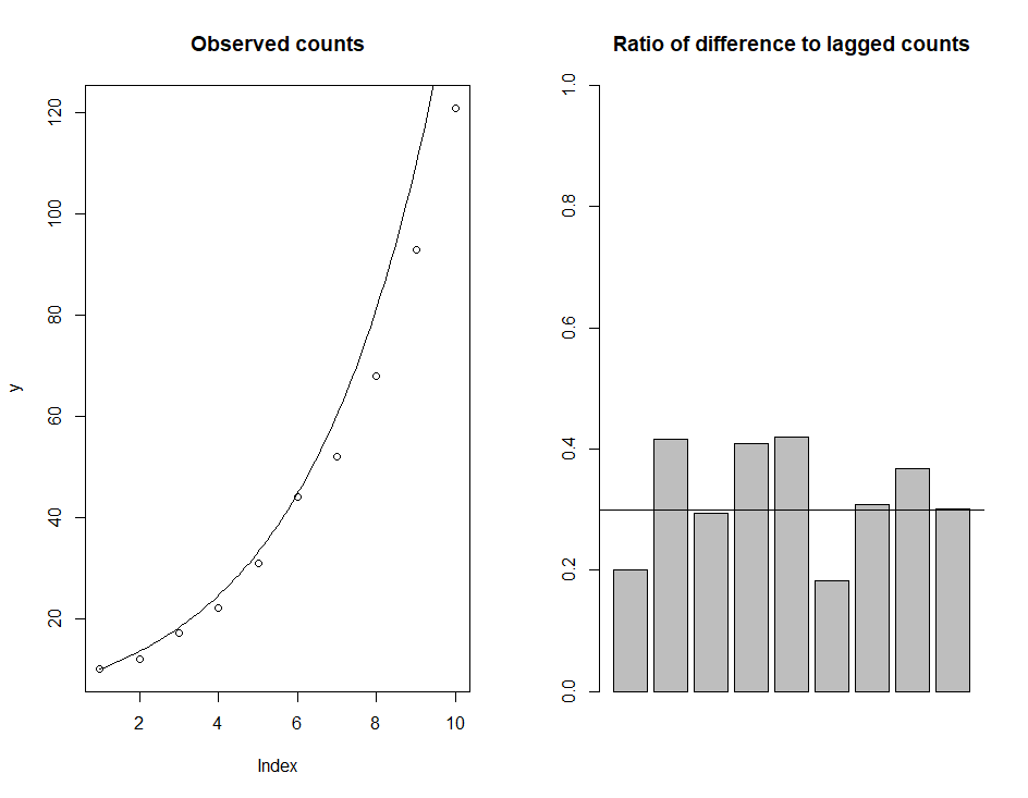
It is not an orthodox approach to population modeling, because you are not estimating the usual logistical model parameters, and I guess the cells are immortal in your assays. But if you express the likelihood in that manner, all you need to do is take the difference of subsequent counts, you can show that they are mutually independent, and multiplied together they express a binomial likelihood. Then you can estimate the parameters for the differential equation expressing the probability model for growth over time.

As an example:

set.seed(123)
r <- 0.3
y0 <- 10
y <- rep(y0, 10)
for(i in 2:length(y)) {
  y[i] <- y[i-1] + rbinom(1, y[i-1], r)
}
dy <- diff(y)
ny <- y[-length(y)]
fit <- glm(cbind(dy,ny-dy) ~ 1, family=binomial(link='identity'))

Provides this estimate:

> fit

Call:  glm(formula = cbind(dy, ny - dy) ~ 1, family = binomial(link = "identity"))

Coefficients:
(Intercept)  
     0.3181  

Degrees of Freedom: 8 Total (i.e. Null);  8 Residual
Null Deviance:      8.532 
Residual Deviance: 8.532    AIC: 43.84

with intuitive graphical depictions of what's actually being measured.