Steps for Forecasting with known copula's parameters

Question

I want to calculate the Mean absolute percentage error (MAPE) for my copula model. I am stuck at the forecasting step. I am not specifying the copula here for different data pairs.

1. I have two time series X and Y. I found the best GARCH parameters $\alpha$ and $\beta$ assuming 0 mean.
2. The Kendals tau between two variables is $\tau$
3. Then I found the best copula and had its parameters say $\kappa$ and $\omega$.
4. Now for forecasting, I need to generate residuals using my copula parameters found in step 3.

How to do this if I want to enter the copula parameters MANUALLY and not use some param=fit type of code in R.

I can work in R as well as Excel. Please if somebody could help me with the exact steps of point 4.

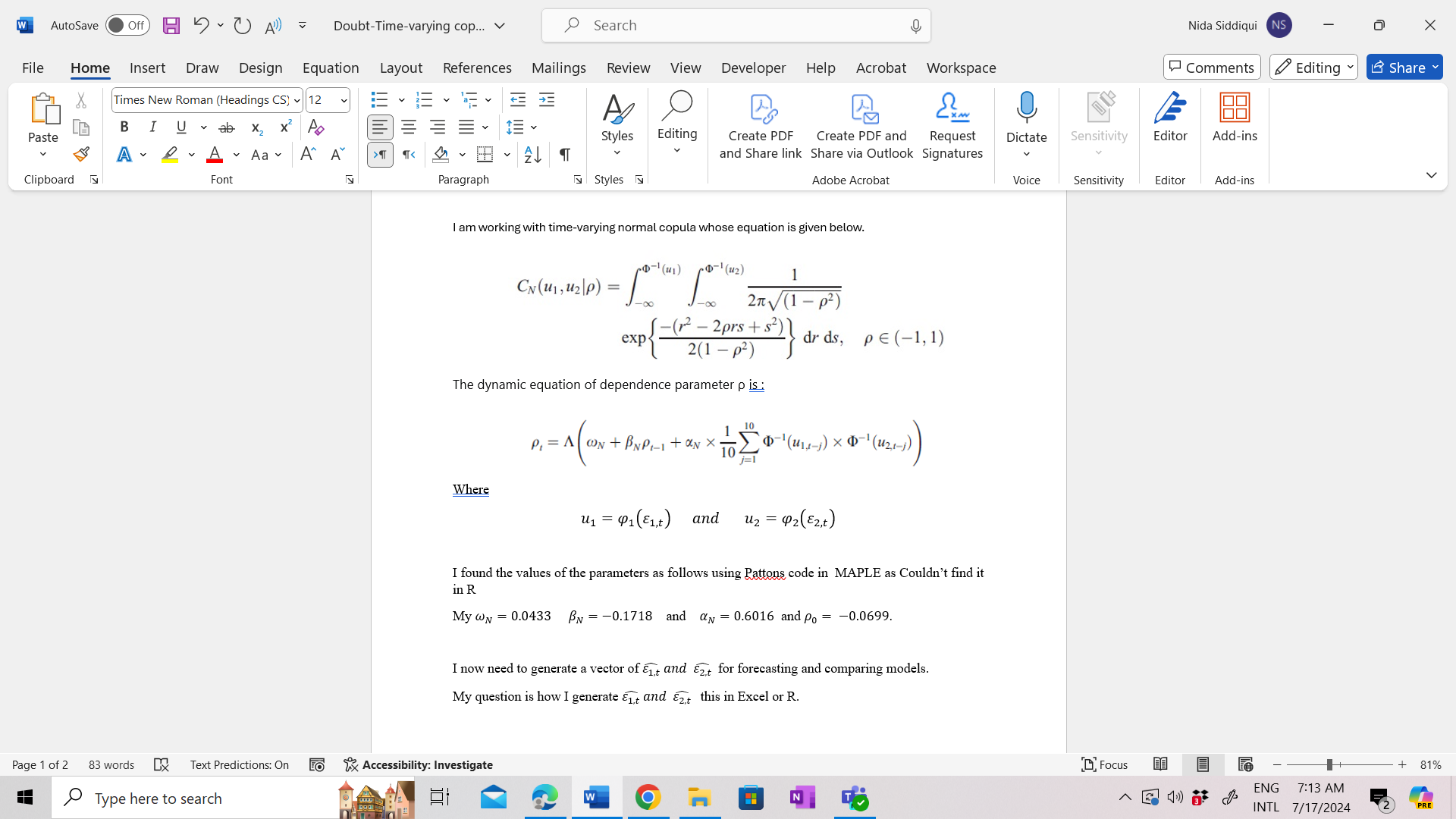
Problem Attachment- More details attachment-

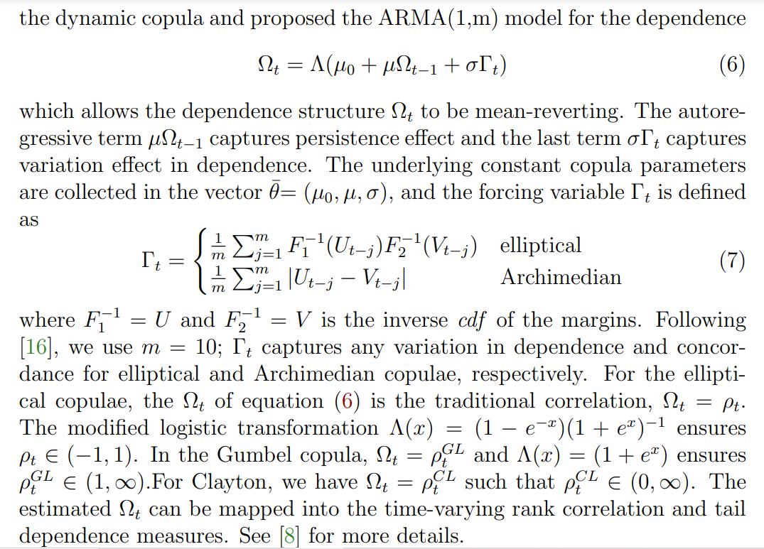
Original paper- Patton (2006)- See page 542

Answer 1

I am unfamiliar with forecasting too much, but it will help based on the provided screenshot. If you want to transform Patton's codes or model from Matlab to R, then you may look at this package. here

In the following code, I first define the necessary parameters and functions based on the information provided in the image. Then, I generate the u1_t and u2_t functions, which are used to calculate the epsilon1_t and epsilon2_t functions. Finally, I generate the vectors epsilon1_vec and epsilon2_vec containing 100 values each, which can be used for forecasting and comparing models.

library(tidyverse)

# Given parameters
w_0 = 0.0433
beta_n = -0.1718
sigma_n = 0.6016
rho_0 = -0.0699

# Time-varying normal copula equation
C_n <- function(u1, u2, p) {
  int1 <- integrate(function(s) exp(-(s^2 - 2*p*s + 1)/(2*(1 - p^2))), 0, u1)$value
  int2 <- integrate(function(s) exp(-(s^2 - 2*p*s + 1)/(2*(1 - p^2))), 0, u2)$value
  (2 * pi * sqrt(1 - p^2))^-1 * exp(-((int1 + int2)/2))
}

# Dynamic equation for dependence parameter p ## you need to muliply it with Λ
p_t <- function(t) {
  w_0 + beta_n*p_t(t-1) + sigma_n * (1/10) * sum(pnorm(u1_t(t-i), 0, 1) * pnorm(u2_t(t-i), 0, 1))
}

# Generating u1_t and u2_t
u1_t <- function(t) pnorm(rnorm(1, 0, 1))
u2_t <- function(t) pnorm(rnorm(1, 0, 1))

# Generating epsilon1_t and epsilon2_t
epsilon1_t <- function(t) -log(-log(u1_t(t)))
epsilon2_t <- function(t) -log(-log(u2_t(t)))

# Generate the vectors for forecasting and comparing models
epsilon1_vec <- sapply(1:100, epsilon1_t)
epsilon2_vec <- sapply(1:100, epsilon2_t)