Predicting daily electricity load - fitting time series

Question

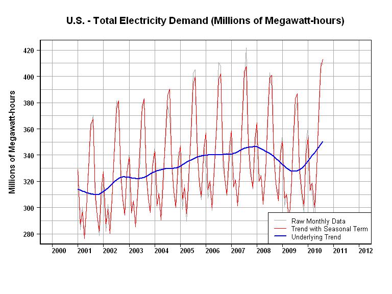
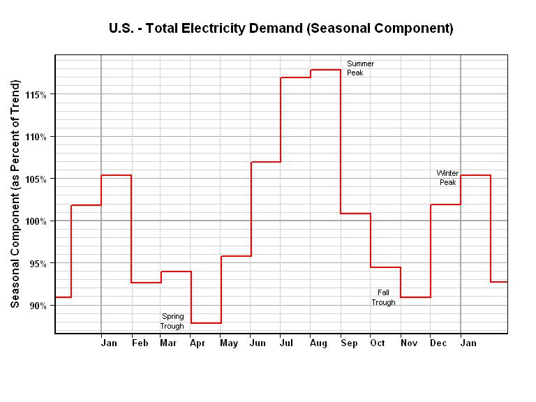
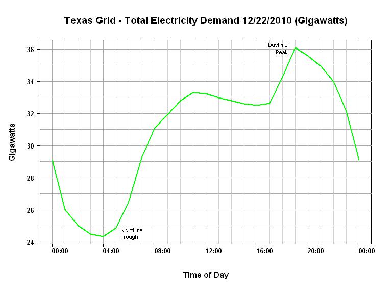
I want to predict inter-day electricity load. My data are electricity loads for 11 months, sampled in 30 minute intervals. I also got the weather-specific data from a meteorological station (temperature, relative humidity, wind direction, wind speed, sunlight). From this, I want to predict the electricity load until the end of the day.

I can run my algorithm until 10:00 of the present day and after that it should give the prediction of loads in 30 minute intervals. So, it should tell the load at 10:30, 11:00, 11:30 and so on until 24:00.

My first attempt was to create a linear model in R.

BP.TS <- ts(Buying.power, frequency = 48)
a <- data.frame(
Time, BP.TS, Weekday, Pressure, Temperature, RelHumidity, AvgWindSpeed, AvgWindDirection, MaxWindSpeed, MaxWindDirection, SunLightTime,
m, Buying.2dayago, AfterHolidayAndBPYesterday8, MovingAvgLast7DaysMidnightTemp
)
a <- a[(6*48+1):nrow(a),]

start = 9716
steps.ahead = 21
par(mfrow=c(5,2))
for (i in 1:10) {
    train <- a[1:(start+(i-1)*48),]
    test <- a[((i-1)*48+start+1):((i-1)*48+start+steps.ahead),]
    summary(reg <- lm(log(BP.TS)~., data=train, na.action=NULL))
    pred <- exp(predict(reg, test))

    plot(test$BP.TS, type="o")
    lines(pred, col=2)
    cat("MAE", mean(abs(test$BP.TS - pred)), "\n")
}

This is not very succesful. Now I try to model the data with ARIMA. I used auto.arima() from the forecast package. These are the results I got:

> auto.arima(BP.TS)
Series: BP.TS 
ARIMA(2,0,1)(1,1,2)[48]                    

Call: auto.arima(x = BP.TS) 

Coefficients:
         ar1      ar2     ma1    sar1     sma1    sma2
      1.1816  -0.2627  -0.554  0.4381  -1.2415  0.3051
s.e.  0.0356   0.0286   0.033  0.0952   0.0982  0.0863

sigma^2 estimated as 256118:  log likelihood = -118939.7
AIC = 237893.5   AICc = 237893.5   BIC = 237947

Now if I try something like:

reg = arima(train$BP.TS, order=c(2,0,1), xreg=cbind(
train$Time, 
train$Weekday, 
train$Pressure, 
train$Temperature, 
train$RelHumidity, 
train$AvgWindSpeed, 
train$AvgWindDirection, 
train$MaxWindSpeed, 
train$MaxWindDirection, 
train$SunLightTime,
train$Buying.2dayago,
train$MovingAvgLastNDaysLoad,
train$X1, train$X2, train$X3, train$X4, train$X5, train$X6, train$X7, train$X8, train$X9, 
train$X11, train$X12, train$X13, train$X14, train$X15, train$X16, train$X17, train$X18, 
train$MovingAvgLast7DaysMidnightTemp
))

p <- predict(reg, n.ahead=21, newxreg=cbind(
test$Time, 
test$Weekday, 
test$Pressure, 
test$Temperature, 
test$RelHumidity, 
test$AvgWindSpeed, 
test$AvgWindDirection, 
test$MaxWindSpeed, 
test$MaxWindDirection, 
test$SunLightTime,
test$Buying.2dayago,
test$MovingAvgLastNDaysLoad,
test$X1, test$X2, test$X3, test$X4, test$X5, test$X6, test$X7, test$X8, test$X9, 
test$X11, test$X12, test$X13, test$X14, test$X15, test$X16, test$X17, test$X18, 
test$MovingAvgLast7DaysMidnightTemp
))

plot(test$BP.TS, type="o", ylim=c(6300,8300))
par(new=T)
plot(p$pred, col=2, ylim=c(6300,8300))
cat("MAE", mean(p$se), "\n")

I get even worse results. Why? I ran out of ideas, so please help. If there is additional information I need to give, please ask.

Answer 1

I've played around with electrical demand models, and I can tell you that it's a good idea to start "zoomed out". Each region has its own characteristics, but the general idea is the same.

Electric demand is a function of many variables. Starting with the slowest moving terms.

1. General Economic Activity is the slowest moving term (typically the 3 to 8 year time frame). This term is typically related to Gross Domestic Product for the area. Electrical Demand may generally grow faster than GDP, but the electrical demand "ups" during good economic times, and demand "downs" during recessions provide an obvious link to GDP. See the blue line in the first graph below.

2. Next, is the Seasonal Term (annual time frame). For instance in the U.S., the Summer Peak shows up in August, the Winter Peak shows up in January, the Spring Trough shows up in April and the Fall Trough shows up in November. See the red line in top two graphs below. In the second graph, I have shown the Seasonal Term to be constant for each month, but you can easily improve that by a linear or non-linear relationship for each month (monthly time frame).

3. You are now down to the daily time frame. The bottom graph shows the Electrical Demand for Texas for one 24 hour period (12/22/2010). The Day-time Peak was at 7:00PM (19:00) and the Night-time Trough was at 4:00AM (04:00). This time frame is where you want to consider holidays, weekends, weather, etc. However, keep in mind that those other variables (in 1 and 2 above) are also affecting your results.

So, from your description, you have data for 11 months. Look at the first graph below and assume that you have data for 11 months. Is that enough to get an idea of the Seasonal Term for the year? I would use a minimum of 10 years of monthly data to get a feel for the Seasonal Term. The idea here is to tweek the structure of your daily model differently during months of "rapid seasonal change" versus months of "slow seasonal change".

Next, I would play around with the size and structure of the "data window" that you will use to estimate your daily model. For example, will you get a better daily model if you include daily fall and winter data when estimating a summer daily model? Or, is it better to use 10 rescaled "summer data windows", one for each year in 10 years of data, when estimating a summer daily model?

Once you get all of the deterministic terms working well, then, and only then would I go after the ARIMA terms.

Answer 2

@Grega:

I ran out of room in the comment area, so I started another answer.

From your comment, that's the problem. Each system/grid has its own "signature". It's a combination of system dynamics, age, weather, local economics, cultures, traditions, etc. In Japan, its worse. Some sections of the country run at 50Hz and other sections run at 60Hz. These grids connect at high voltage DC stations, which means some areas behave like electrical "islands" (totally different behavior than their neighbors just a few miles away). If you're zeroed-in on one factory, the predictability goes down even more. Fewer users means higher uncertainty.

No matter how you do this, it's going to be messy.

I would filter out the daily/weekday/weekend/holiday component to get a Seasonal Term. How? A 31 day CENTERED moving average? 51 day CMA? XX day CMA? You'll have to experiment with that, but I would make it a variable so you can tweek it later. Whatever filter you end up with, keep in mind that it stops short of either end of your data (a 31 day centered moving average will start on the 16th day of your raw data and end on the 16th day from the end of your raw data).

Next, the best you can do with 11 months of data is to "make up" month 12 (draw a line from your filtered series at its end to its beginning). Next, subtract your Seasonal Term (the filtered data) from your raw data to get a residual. Fit the residual to your weather data, allowing for factors for day-of-the-week and holidays.

Some factors that you may need to add are:

1) A "production run" factor. Whatever they make at this factory, if they switch from one product/category to another, the power demand required to make one product may be different than what is required for another product.

2) A "change over" factor. This is when they shift from one product/category to another. Sometimes it takes days of preparation for the switch.

3) A "work shift" factor. If they have three shifts per day, power demand for the late shift will probably be significantly different than the day shifts.

Good luck. As you probably know, this kind of a problem can get real frustrating.

====== Edit to answer Grega's first comment (01/25/2011) ====================

@Grega: Answering your first comment, I'm afraid it doesn't. The idea behind a model like this would be to have multiple "similar instances" of your 32 future points, so you can fit those points, and then predict new points. You don't have typical "similar instances" because yesterday was not the same day-of-the-week as today. You have to use last week's same day-of-the-week and the previous week's same day-of-the-week, etc. By the time you get several "similar instances" (say 20), you're typically more than 20 weeks in the past (a holiday may screw up one or more of your weeks). At that point, you're in a whole different season of the year. So, in order to use those days in another season, you need to remove the Seasonal Term from the raw data.

It's a sloppy situation, but it's the best you can do with 11 months of data.