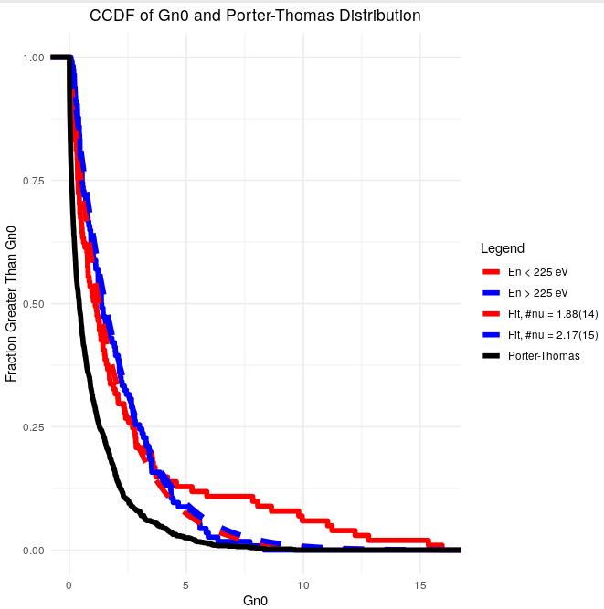
I have two data sets (let call them L and G) that represent a measured physical quantity $\Gamma_n^0(\delta\Gamma_n^0)$. I am performing a Kolmogorov-Smirnov test in R between these two datasets which yields a p-value of 4.68e-6. That means these data sets come from different distributions (cross checking my understanding).
I expect each distribution to follow the Porter-Thomas distribution (PTD) (i.e. a chi-square distribution with one degree of freedom). I test my two data sets again the PTD and I get 2.904e-06 for the L dataset and 1.461e-12 for the G dataset. Although this is against what I was expecting in the beginning, it's exciting information so it's not a problem.
Then I wanted to fit these two datasets with a chi-square distribution to extract the number of degrees of freedom. I used a maximum likelihood fit. The L dataset fit yielded 1.88(15) degrees of freedom and the G 2.17(15). The fits don't contradict the KS test of the datasets again the PT distribution.
However, the fits show compatible (within uncertainties) degrees of freedom. To me this means that they come from the same distribution which contradicts the KS test against the data sets!
I would like to understand if I can trust the KS test more the fits, or the fits more than the KS tests.
For reference in neither the fits or the KS test, I'm not using my uncertainties. I know I should, I just don't know how.
Also, this is a plot that summarizes some of the above tests (fits in dashed lines, L is En<225 and G is En>225).
Also here is the code I am using in R to do these calculations, in case it's helpful!
#______________________________________________________________________________________________________
# (0) Load libraries

library(dplyr)
library(stats)
library(ggplot2)
library(kSamples)
library(twosamples)
library(MultNonParam)
library(fitdistrplus)


#______________________________________________________________________________________________________
# (1) General parameters/variables

i = 1/2 #neutron spin i
I = 7/2 #target nucleus spin I
terminal_width <- getOption("width")

# Porter-THomas
n  <- 1000  # Number of samples to generate for the Porter-Thomas distribution
set.seed(123)  # For reproducibility
porter_thomas <- rchisq(n, 1)

#______________________________________________________________________________________________________
# (2) Read the data, using the first line as the header and calculate other useful quantities

# in the final pub file I have removed negative energies and all widths are positives
data = read.table("149Sm_resonance_parameters_FINAL_pub.dat", header=TRUE, sep="")
data_filtered = data %>% mutate(Gn0   = Gn / sqrt(En),
                                         dGn0  = sqrt((1 / sqrt(En) * dGn)^2 + (-Gn / (2 * En^(3/2)) * dEn)^2),
                                         g     = (2*J+1)/(2*i+1)/(2*I+1),
                                         gGn   = g*Gn,
                                         dgGn  = g*dGn,
                                         gGg   = g*Gg,
                                         dgGg  = g*dGg,
                                         gGn0  = g*Gn0,
                                         dgGn0 = g*dGn0
                                        )
#print(data_filtered)

#______________________________________________________________________________________________________
# (3) Get the data to perform the statistical tests later
Gn0_LT_225 = data_filtered %>% filter(En < 225 & Gn != 0 & dGn != 0)
Gn0_GT_225 = data_filtered %>% filter(En > 225 & Gn != 0 & dGn != 0)

#______________________________________________________________________________________________________
# (5) Statistical analysis of Gn

cat(strrep("_", terminal_width), "\n")
cat("Statistical analysis of Gn\n\n\n")

# Kolmogorov-Smirnov test
ks_test <- ks.test(Gn0_LT_225$Gn, Gn0_GT_225$Gn)
print(ks_test)
cat("\n")

ks_test <- ks.test(Gn0_LT_225$Gn0, porter_thomas)
print(ks_test)
cat("\n")

ks_test <- ks.test(Gn0_GT_225$Gn0, porter_thomas)
print(ks_test)
cat("\n")

# Fit chi-square distribution to Gn0_LT_225 data
fit_LT_225 <- fit_chisq(Gn0_LT_225$Gn0)
print(fit_LT_225)

# Fit chi-square distribution to Gn0_GT_225 data
fit_GT_225 <- fit_chisq(Gn0_GT_225$Gn0)
print(fit_GT_225)

# Extract the estimated degrees of freedom
df_LT_225 <- fit_LT_225$estimate["df"]
df_GT_225 <- fit_GT_225$estimate["df"]

print(paste("Estimated df for Gn0_LT_225:", df_LT_225))
print(paste("Estimated df for Gn0_GT_225:", df_GT_225))

# Plot the fit
x11()
plot(fit_LT_225)

x11()
plot(fit_GT_225)

# Define a sequence of x values for plotting the chi-square fits
x_vals <- seq(min(c(Gn0_LT_225$Gn0, Gn0_GT_225$Gn0)), max(c(Gn0_LT_225$Gn0, Gn0_GT_225$Gn0)), length.out = 1000)

# Calculate the fitted chi-square CDFs
fitted_LT_225 <- pchisq(x_vals, df = df_LT_225)
fitted_GT_225 <- pchisq(x_vals, df = df_GT_225)

# Convert to data frame for plotting
fitted_df <- data.frame(x = x_vals,
                        fitted_LT_225 = 1 - fitted_LT_225,
                        fitted_GT_225 = 1 - fitted_GT_225,
                        porter_thomas_fit = 1 - porter_thomas_fit)

# Plot the empirical distributions and the fits
comparison_plot <- ggplot() +
  # Empirical CCDF of Gn0_LT_225 values
  stat_ecdf(data = Gn0_LT_225, aes(x = Gn0, y = 1 - after_stat(y), color = "En < 225 eV"), linewidth = 2) +
  # Empirical CCDF of Gn0_GT_225 values
  stat_ecdf(data = Gn0_GT_225, aes(x = Gn0, y = 1 - after_stat(y), color = "En > 225 eV"), linewidth = 2) +
  # Fitted CCDF of Gn0_LT_225 values
  geom_line(data = fitted_df, aes(x = x, y = fitted_LT_225, color = "Fit, #nu = 1.88(14)"), linewidth = 2, linetype = "dashed") +
  # Fitted CCDF of Gn0_GT_225 values
  geom_line(data = fitted_df, aes(x = x, y = fitted_GT_225, color = "Fit, #nu = 2.17(15)"), linewidth = 2, linetype = "dashed") +
  # Porter-Thomas distribution
  stat_ecdf(data = porter_thomas_df, aes(x = Gn0, y = 1 - after_stat(y), color = "Porter-Thomas"), linewidth = 2) +
  labs(title = "CCDF of Gn0 and Porter-Thomas Distribution",
       x = "Gn0",
       y = "Fraction Greater Than Gn0",
       color = "Legend") +
  scale_color_manual(values = c("En < 225 eV" = "red",
                                "En > 225 eV" = "blue",
                                "Fit, #nu = 1.88(14)" = "red",
                                "Fit, #nu = 2.17(15)" = "blue",
                                "Porter-Thomas" = "black")) +
  theme_minimal() +
  theme(plot.title = element_text(hjust = 0.5),
        #legend.position = "bottom", # Move legend to bottom
        #legend.box = "horizontal", # Arrange legend items horizontally
        #legend.box.spacing = unit(1, "cm"), # Space between legend boxes
        #legend.key.width = unit(1.5, "cm"), # Width of legend keys
        #legend.key.height = unit(0.5, "cm"), # Height of legend keys
        #legend.text = element_text(size = 10), # Adjust text size
        #legend.title = element_text(size = 12) # Adjust title size
       )

# Print the plot
dev.new()
print(comparison_plot)

