Accounting for non-independence and autocorrelation in HGAM

Question

I am currently trying to fit a HGAM to model differences in daily activity patterns of fish in two treatments. Data were collected with high-resolution telemetry, and I currently have estimates of total distance swum (m) per hour (1-24) for 30 fish (~15 of each treatment) over the course of ~35 experimental days for each of three lakes (lakes A-C).These data have a clear hierarchical structure, which I am trying to account for with random effects (please let me know if my syntax is wrong as I am used to modelling in brms /lme4 ). I am creating a separate model for each lake to reduce model complexity. The model structure is as follows:

mod <- gam(as.numeric(total_distance) ~ 
               Treatment + exp_day_z + weight_z +
               s(hour, by = Treatment, k = 22, bs = "cc") + # this is my interaction of interest
               s(individual_ID, bs = 're') + # individual-level random intercept
               s(individual_ID, exp_day_z, bs = 're') + # individual-level random slope for experimental day (centred)
               s(individual_ID, hour, bs = 're'), # individual-level random slope for hour
            data = filter(perch, lake == 'A'),
            method = "REML",
            knots=list(hour=c(0.5, 24.5)),
            family = Gamma(link = 'log'))

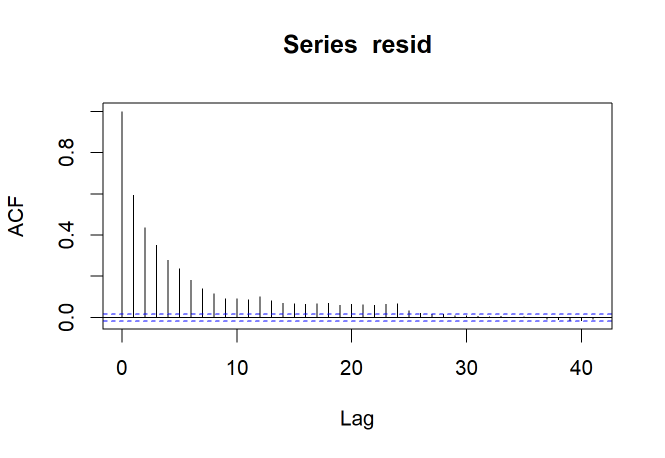
However, there still seems to be substantial autocorrelation in the residuals.

After reading Eric Pedersen's HGAM paper, watching several of his and Gavin Simpson's great tutorials, and reading a few older posts, I decided to try an autoregressive term in the model to account for this, as follows:

perch <- perch %>%
  arrange(individual_ID, exp_day, hour) %>%
  mutate(start = if_else(is.na(lag(individual_ID)) | individual_ID != lag(individual_ID), TRUE, FALSE))

mod2 <- bam(as.numeric(total_distance) ~ 
               Treatment + exp_day_z + weight_z +
               s(hour, by = Treatment, k = 22, bs = "cc") + 
               s(individual_ID, bs = 're') +
               s(individual_ID, exp_day_z, bs = 're') +
               s(individual_ID, hour, bs = 're'),
            data = filter(perch, lake == 'A'),
            method = "fREML",
            rho = 0.6,
            AR.start = start,
            discrete = TRUE,
            knots=list(hour=c(0.5, 24.5)),
            family = Gamma(link = 'log'))

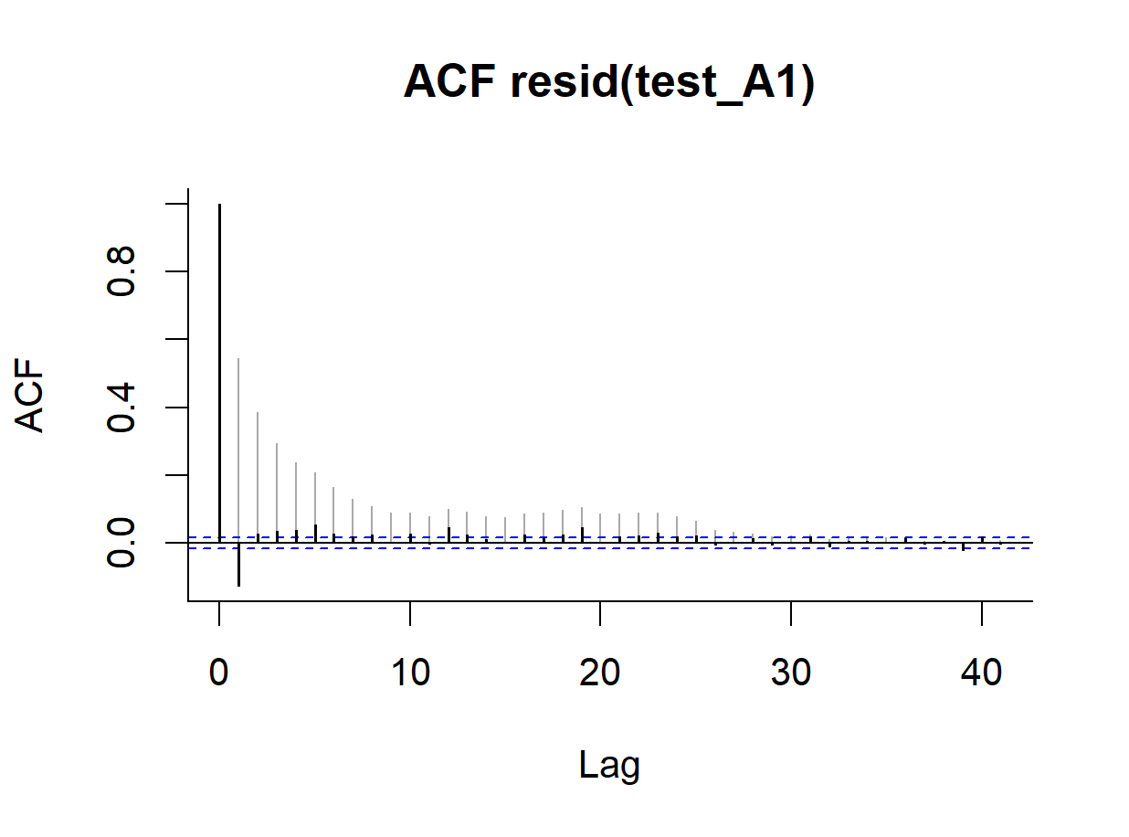
This seemed to improve the residual autocorrelation (note: this acf plot was generated with check_resid(mod2) where grey bars represent standard residuals and black bars denote standardized AR1 corrected residuals).

This model also seemed to produce sensible predictions with slightly wider CI's than my previous model (note: contrasts were estimated using the comparisons function from the marginaleffects package).

I am still a little unsure of a few things:

1. Should I be including random effects and an autoregresive term in the same model?
2. Is my random effects structure formatted correctly, where hour and experimental day are individual-level random slopes?
3. What is the rationale for choosing specific rho values when using the bam() function?
4. Finally, somewhat unrelated, is there a way to get lake- and treatment-specific smooths from one overall model, rather than model the three lakes separately (I initially tried to do this with by = Interaction(Treatment, lake) but this took ages to run, but perhaps this is the only way)?

Any help would be greatly appreciated!

Thanks

Answer 1

1. Yes, this is OK; both terms will model variation among observations.

2. I don't think you have the ranef specification right; why do you think that globally the hour effect is smooth, but individually the effect is linear?

   I would suggest using "random" splines for the hour ranef:

   s(hour, individual_ID, bs = "fs", xt = list(bs = "cc"))
   

3. $\rho$ is the parameter of the AR(1) process you are fitting alongside the other model terms. You need to supply this parameter such that the model can estimate the other smooth and parametric effects conditional on the specified AR(1) term in the covariance. You can usually read off the value of this parameter from the ACF at lag 1 (which is the correlation of the residuals with itself lagged 1 time step). Be sure to compute the ACF correctly - you can't just do an ACF on the entire set of residuals because you have multiple time series, one per individual. Instead, extract residuals and split them up by individual_ID and fit the ACF for each individual and then take the average of the values for the lag-1 correlation as your guess for $\rho$

4. I would suggest fitting your lake-specific model using the "sz" basis:

   total_distance ~ 
     exp_day_z + weight_z +
     s(hour, k = 22, bs = "cc") +
     s(hour, Treatment, k = 22, bs = "sz", xt = list(bs = "cc")) +
     ...
   

   In which we get the same thing as your version but we get it in a way that is better than the by option for global plus group smooths from our HGAM paper. This "sz" basis wasn't available in mgcv when we wrote the HGAM paper so that paper represents best practice (according to us) at the time. Now, the "sz" basis is cleaner because the "sz" basis is explicitly orthogonal to the "main" effect smooth.

   This allows easy extension to the multi-lake model:

    total_distance ~ 
      exp_day_z + weight_z +
      s(hour, k = 22, bs = "cc") +
      s(hour, Treatment, k = 22, bs = "sz", xt = list(bs = "cc")) +
      s(hour, Lake, k = KK, bs = "sz", xt = list(bs = "cc")) +
      s(hour, Treatment, Lake, k = KK, bs = "sz", xt = list(bs = "cc")) +
      ...
   

   Where we have main effects of hour, interaction with Treatment and Lake, plus the third order of hour, treatment, and lake. KK here is just to highlight you need to specify something here if you want something other than the default; but remember that these "sz" smooths are true difference smooths, so you likely don't want to have as complex differences as you have for the hourly smooth and hence don't need k as high for the "sz" smooths.

   You can do this model with your by approach, but often it is more parsimonious to use the "sz" version:

    # make the interaction in the data
    perch <- perch |>
      transform(
        lake_treatment = interaction(Treatment, lake, drop = TRUE)
      )
   
    ...
   
    total_distance ~ 
      exp_day_z + weight_z + lake_treatment +
      s(hour, by = lake_treatment, k = 22, bs = "cc") +
      ...
   

The "sz" model is more like a linear model for different orders of interactions, with main effects and interaction terms. The by model in the way you are fitting it simply fits one smooth of hour per combination of Treatment of lake; hence from the model itself, the "sz" one allows you see in the model terms themselves which interactions are important. You can't do this just from the model terms in the by variant as they simply code for lake:treatment smooths themselves, not deviations. With the "sz" version then, the summary would give you a test of the effects of Treatment and lake.

FYI: your knots argument is wrong. 00:00 is the same as 24:00 hours, hence you want knots = c(0, 24) as that's where the circular covariate wraps back on itself, and any values outside the range [0-24] are not possible.

Answer 2

On top of Gavin's answer I'll add that you can use the {mvgam} package if you need to allow each fish to have a potentially different $\rho$ parameter. The package allows all of the same effects that you want to use in gam() or bam() so hopefully it won't be too much of a learning curve. You could of course then expand up to more complex latent dynamics should you need them, such as higher order AR terms with correlated errors, Vector Autoregressions or dynamic factors, which might be helpful for capturing the types of multivariate processes that likely occur in your data.