Random number generation and probability

Question

I recently ran into two problems:

1. given a rand() function that generates 0 and 1 with 50% probability respectively (binary outcome), how to write some code to generate 1 with 90% of the chance and 0 with 10%?

2. There is a society where people will NOT stop having babies until they have a boy. What's the ratio of boys and girls in that society? Consider it's equal probability to have either a boy or a girl.

If possible, please advise what kind of background prob/stats materials these relate to. Thanks!

UPDATE: Here are some thoughts on the two questions:

1.since rand() only generate 0 or 1, it's useless to write code like the following:

if (rand() < 0.1) {
     return 0;
} else {
     return 1;
}

I guess this involves Bernoulli trial and Binomial distribution, but the question asks for EXACT distribution for 90% of 1 and 10% of 0. I'm puzzled how to proceed.

2.I put it the wrong way - my bad. My initial thoughts on this is as follows:

Suppose $\text{P}(B) = \text{P}(G) = 0.5$
B' = boys in the society

$$\text{P}(B') = \text{P}(B) + \text{P}(B|G) + \text{P}(B|G,G) + \text{P}(B|G,G,G) + ...$$

But I didn't see how to derive this equation into computable format.

UPDATE 2 (from @David Marx):

1. Problem 1

   think of this as a binary number with 4 bits (n) - represents range [0, 15] with each equal probability of 1/16. Now to get 1 with 90% probability, we can write something like this:

   if (n < 9) { return 1; } else if (n == 9) { return 0; }

This way, Prob(n in range[0,9)) = 9/16; Prob(n = 9) = 1/16; So the returned value will be 1 at 90% of the time.

1. Problem 2

The reminding of Geometric Series is appreciated! The equation indeed matches my initial thoughts on the summation of conditional probabilities -- I failed to recognize it as geometric series.

So I guess the ratio should be the result for that summation:

$$\text{P}(B') = (1/2) + (1/2)^2 + (1/2)^3 + ... = 1/(1-(1/2)) - 1 = 1. $$

So the ratio of boys in the society will be 100%? Anything wrong here?

Answer 1

The answer to the second question is that the ratio becomes undefined because the society has a 100% chance of dying out. The reason why this happens is fascinating: statistical fluctuations in the balance of males and females (a "second order effect") in a population that otherwise would appear to be stable in size (a "first order effect") will cause it to decrease.

---

Analysis

To make it clear what this statement means, here are the assumptions I use:

• The "society" (let's just call it a population because it acts in a very non-human way) consists of males and females, all of which might potentially breed.

• Breeding is performed by associating males and females permanently into as many pairs as possible. Each pair produces one offspring sequentially.

• A pair produces males with 50% probability, independently with each birth and independently of all other pairs.

• Breeding for a pair stops when either (a) a male is produced or (b) a predetermined finite limit $l$ of offspring is reached. (The latter is a necessary nod to realism: no individual is immortal!)

• After all pairs stop breeding, the new generation commences breeding in the same way. (That is, there is no overlap of generations and no pairing between generations.)

Under these assumptions, all relevant information is conveyed by the number of males $M$ and number of females $F$ in the current generation. The number of breeding pairs equals $\min(M,F)$. Each pair produces one male (unless it reaches the limit) and a number of females according to a geometric distribution. This is a truncated geometric distribution for the number of females. If there were no limit, it would be a geometric distribution where the probability of $F$ females is

$$\begin{align} \Pr(F=0) &= 1/2 \\ \Pr(F=1) &= 1/4 \\ \cdots \\ \Pr(F=k) &= 2^{-k-1} \\ \cdots \end{align} $$

Because there is a limit, this list stops with $\Pr(F=l) = 2^{-l-1} + 2^{-l-2} + \cdots = 2^{-l}$. Consequently the expected number of males per breeding pair is

$$ \mathbb{E}[M] = \left(1/2 + 1/4 + \cdots + 2^{-l} + 0 \times 2^{-l}\right) =1 - 2^{-l}. $$

and the expected number of females can similarly be computed. It is clear that in a large population, because the expected number of males is less than one per breeding pair, the expected number of breeding pairs is less in each generation.

Furthermore--regardless of whether we include a limit in the model--variation in the numbers of males and females will cause the population eventually to die out anyway. This is because the number of breeding pairs can only equal the smaller of the numbers of males or females produced in the preceding generation and fluctations in both of those (which are up or down from the expected value with roughly equal probability) will cause the smaller of the two to fluctuate downwards much more often than it fluctuates upwards. This mechanism further forces the population down to zero.

---

Experiments

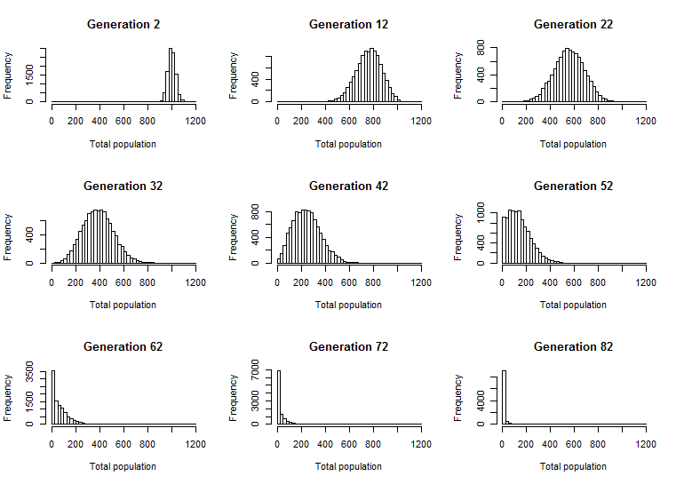
Rather than carry out a full and rigorous analysis of the effects of fluctuation, let's do a simulation and look at what happens to small populations of, say, $500$ males and $500$ females. I did this calculation $10,000$ separate times for $81$ new generations (setting the limit to an infinite value, to be conservative):

Clearly the continuation of this population is hopeless: although initially there is some chance that it increases, inevitably the population shrinks. The shrinking quickly is evident: within $12$ new generations, there is almost no chance the latest generation exceeds the size of the first generation (of $1000$). There is almost no chance this particular population will last more than $100$ generations.

(Larger populations will take more than $12$ generations to shrink with near certainty, but the same things eventually happen to them.)

---

Here is R code to perform the simulation.

next.gen <- function(pop, p=1/2, limit=30) {
  n.females <- rgeom(n <- min(pop), p)
  has.male <- n.females <= limit
  return(c(males=sum(has.male), 
           females=sum(n.females[has.male]) + sum(rep(limit, n)[!has.male])))
}
simulate <- function(pop, n=1, ...) {
  result <- matrix(0, nrow=n, ncol=2)
  colnames(result) <- c("males", "females")
  n.gen <- 1; k <- 0
  while(n.gen <= n && sum(pop <- result[n.gen,] <- next.gen(pop, ...)) > 0) 
    {n.gen <- n.gen+1}
  return(result)
}
pop <- c(males=500, females=500)
set.seed(17)
system.time(d <- replicate(10^4, rowSums(simulate(pop, 81, limit=Inf))))
par(mfrow=c(3,3))
tmp <- sapply(seq(1,81,10), function(i) hist(d[i,], breaks=seq(0,1200,25),
                                    main=paste("Generation", i+1),
                                    xlab="Total population"))

Answer 2

Here are some thoughts to get you started:

Problem 1

The probability of getting a single 1 (or 0) is 50%, and as you've noticed this isn't especially helpful. But what's the probability of getting 00 in two trials? or 010 in three trials? Or at least two 1's in four trials? I'd recommend you start thinking about what you can accomplish if you shift your event space from single events to sequences of experiments. From there, you can look at permutations, combinations, minimal conditions... You can also combine probabilities using AND and OR rules, or even conditional probabilities.

UPDATE: Regarding your current solution, when in doubt: run some simulations and see what happens!

N=1e7
experiments = sample(1:16, N, replace=T)
viable = experiments[experiments <10]
mean(viable<9) #.8888 ~ 8/9

Hmmm... not quite $9/10ths$. Why do you suppose we got $8/9ths$ instead? You're almost there! Also, as whuber mentioned, the direction you are going is not the only solution to this problem. But what you're doing is creative and I think you should stay the course before figuring out a method that doesn't require you to drop samples.

Nevermind, your solution for this part actually works. I forgot that you were counting up from 0 and not 1. Good job! Now work on making whuber happy :)

Problem 2

The number of trials required to achieve a single success can be modeled using a Geometric Distribution. I don't want to give away the whole solution here, but take a look at the calculation for the mean (i.e. the "expected value") for this distribution given a known success probability.

UPDATE: I was suggesting you look at the mean of the geometric distribution, not use ageometric series (well, in all fairness, they're definitely closely related). Your geometric series calculation contains the entire sampling space, so we should expect it to sum to 1 (you're basically on track to derive the pdf of the geometric distribution). Also, just intuitively, you should see why the expected ratio absolutely should not be 100% boys. We're not precluding female births here in any way.

Answer 3

The second problem has been discussed in Mathematics StackExchange (https://math.stackexchange.com/questions/218674/ratio-of-boys-and-girls) and in MathOverflow (https://mathoverflow.net/questions/17960/google-question-in-a-country-in-which-people-only-want-boys and https://mathoverflow.net/questions/132297/boys-and-girls-revisited). There seems to be disagreement about what the "correct" answer is; it depends on how you interpret the question.