This question has a nice visual solution, because $X$ essentially is the "percentage point function" or "inverse CDF" given by $F^{-1}.$
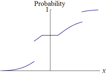
Let's begin with the graph of a generic distribution function $F$:

The general problem illustrated by this plot is that $F$ has no inverse, because (a) its range misses large portions of the interval $[0,1]$, corresponding to the jumps in the graph, and (b) there is an interval of values associated with the same probability, corresponding to the flat region crossing the vertical axis.
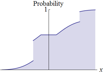
We may fix (a) by filling in the region between the graph and the value axis:

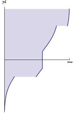
The boundary of this region defines an invertible function from the probabilities $[0,1]$ to the support of $F.$ As usual, flip the axes to plot the inverse relation (which I have done by rotating the plot and displaying it from behind):

The horizontal axis depicts "probability space" $[0,1]$ while the vertical axis now depicts the real numbers, or "value space." Due to problem (b) the boundary of the shaded region isn't quite the graph of a function: it has a vertical segment in the middle. That segment spans a set of values with no probability. Except at its endpoints, it doesn't correspond to anything in the support of $F.$ We may therefore select one point in the span, such as the highest point.
The resulting graph plots the random variable $X$ being sought. You will need to verify that it is measurable (which follows from the definition of $F$), but the most important calculation is to establish that the probability law of $X$ really is $F$: namely, that for any $x\in\mathbb{R},$
$$\Pr(X\le x) = F(x).$$
But this is immediate, because the event $X\le x$ consists of all values $p\in[0,1]$ for which $p \le F(x),$ which has probability equal to the length of the interval $[0,F(x)]$ (that is, the Lebesgue measure of $X^{-1}((-\infty, x])$), which obviously is $F(x).$

