Combining information from multiple studies to estimate the mean and variance of normally distributed data - Bayesian vs meta-analytic approaches

Question

I have reviewed a set of papers, each reporting the observed mean and SD of a measurement of $X$ in its respective sample of known size, $n$. I want to make the best possible guess about the likely distribution of the same measure in a new study that I am designing, and how much uncertainty is in that guess. I am happy to assume $X \sim N(\mu, \sigma^2$).

My first thought was meta-analysis, but the models typically employed focus on point estimates and corresponding confidence intervals. However, I want to say something about the full distribution of $X$, which in this case would also including making a guess about the variance, $\sigma^2$.

I have been reading about possible Bayeisan approaches to estimating the complete set of parameters of a given distribution in light of prior knowledge. This generally makes more sense to me, but I have zero experience with Bayesian analysis. This also seems like a straightforward, relatively simple problem to cut my teeth on.

1) Given my problem, which approach makes the most sense and why? Meta-analysis or a Bayesian approach?

2) If you think the Bayesian approach is best, can you point me to a way to implement this (preferably in R)?

Related question

EDITS:

I have been trying to work this out in what I think is a 'simple' Bayesian manner.

As I stated above, I am not just interested in the estimated mean, $\mu$, but also the variance,$\sigma^2$, in light of prior information, i.e. $P(\mu, \sigma^2|Y)$

Again, I know nothing about Bayeianism in practice, but it didn't take long to find that the posterior of a normal distribution with unknown mean and variance has a closed form solution via conjugacy, with the normal-inverse-gamma distribution.

The problem is reformulated as $P(\mu, \sigma^2|Y) = P(\mu|\sigma^2, Y)P(\sigma^2|Y)$.

$P(\mu|\sigma^2, Y)$ is estimated with a normal distribution; $P(\sigma^2|Y)$ with an inverse-gamma distribution.

It took me a while to get my head around it, but from these links(1, 2) I was able, I think, to sort how to do this in R.

I started with a data frame made up from a row for each of 33 studies/samples, and columns for the mean, variance, and sample size. I used the mean, variance, and sample size from the first study, in row 1, as my prior information. I then updated this with the information from the next study, calculated the relevant parameters, and sampled from the normal-inverse-gamma to get the distribution of $\mu$ and $\sigma^2$. This gets repeated until all 33 studies have been included.

# Loop start values values

  i <- 2
  k <- 1

# Results go here

  muL      <- list()  # mean of the estimated mean distribution
  varL     <- list()  # variance of the estimated mean distribution
  nL       <- list()  # sample size
  eVarL    <- list()  # mean of the estimated variance distribution
  distL    <- list()  # sampling 10k times from the mean and variance distributions

# Priors, taken from the study in row 1 of the data frame

  muPrior  <- bayesDf[1, 14]    # Starting mean
  nPrior   <- bayesDf[1, 10]    # Starting sample size
  varPrior <- bayesDf[1, 16]^2  # Starting variance

  for (i in 2:nrow(bayesDf)){

# "New" Data, Sufficient Statistics needed for parameter estimation

    muSamp    <- bayesDf[i, 14]          # mean
    nSamp     <- bayesDf[i, 10]          # sample size
    sumSqSamp <- bayesDf[i, 16]^2*(nSamp-1)  # sum of squares (variance * (n-1))

# Posteriors

    nPost   <- nPrior + nSamp
    muPost  <- (nPrior * muPrior + nSamp * muSamp) / (nPost)  
    sPost   <- (nPrior * varPrior) + 
                sumSqSamp + 
               ((nPrior * nSamp) / (nPost)) * ((muSamp - muPrior)^2)
    varPost <- sPost/nPost
    bPost   <- (nPrior * varPrior) + 
                sumSqSamp + 
               (nPrior * nSamp /  (nPost)) * ((muPrior - muSamp)^2)
# Update 

    muPrior   <- muPost
    nPrior    <- nPost
    varPrior  <- varPost

# Store

    muL[[i]]   <-  muPost
    varL[[i]]  <-  varPost
    nL[[i]]    <-  nPost
    eVarL[[i]] <- (bPost/2) / ((nPost/2) - 1)

# Sample

    muDistL  <- list()  
    varDistL <- list()

    for (j in 1:10000){
      varDistL[[j]] <- 1/rgamma(1, nPost/2, bPost/2)
      v             <- 1/rgamma(1, nPost/2, bPost/2)
      muDistL[[j]]  <- rnorm(1, muPost, v/nPost)
    }

# Store 

    varDist    <- do.call(rbind, varDistL)
    muDist     <- do.call(rbind, muDistL)
    dist       <- as.data.frame(cbind(varDist, muDist))
    distL[[k]] <- dist

# Advance

    k <- k+1 
    i <- i+1

  }

  var     <- do.call(rbind, varL)
  mu      <- do.call(rbind, muL)
  n       <- do.call(rbind, nL)
  eVar    <- do.call(rbind, eVarL)
  normsDf <- as.data.frame(cbind(mu, var, eVar, n)) 
  colnames(seDf) <- c("mu", "var", "evar", "n")
  normsDf$order <- c(1:33)

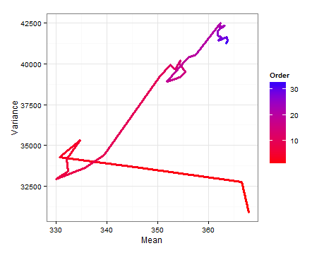
Here is a path diagram showing how the $E(\mu)$ and $E(\sigma^2)$ change as each new sample is added.

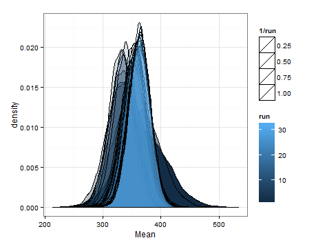
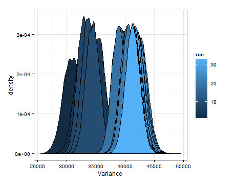
Here are the desnities based on sampling from the estimated distributions for the mean and variance at each update.

I just wanted to add this in case it is helpful for someone else, and so that people in-the-know can tell me whether this was sensible, flawed, etc.

Answer 1

The two approaches (meta-analysis and Bayesian updating) are not really that distinct. Meta-analytic models are in fact often framed as Bayesian models, since the idea of adding evidence to prior knowledge (possibly quite vague) about the phenomenon at hand lends itself naturally to a meta-analysis. An article that describes this connection is:

Brannick, M. T. (2001). Implications of empirical Bayes meta-analysis for test validation. Journal of Applied Psychology, 86(3), 468-480.

(the author uses correlations as the outcome measure for the meta-analysis, but the principle is the same regardless of the measure).

A more general article on Bayesian methods for meta-analysis would be:

Sutton, A. J., & Abrams, K. R. (2001). Bayesian methods in meta-analysis and evidence synthesis. Statistical Methods in Medical Research, 10(4), 277-303.

What you seem to be after (in addition to some combined estimate) is a prediction/credibility interval that describes where in a future study the true outcome/effect is likely to fall. One can obtain such an interval from a "traditional" meta-analysis or from a Bayesian meta-analytic model. The traditional approach is described, for example, in:

Riley, R. D., Higgins, J. P., & Deeks, J. J. (2011). Interpretation of random effects meta-analyses. British Medical Journal, 342, d549.

In the context of a Bayesian model (take, for example, the random-effects model described by equation 6 in the paper by Sutton & Abrams, 2001), one can easily obtain the posterior distribution of $\theta_i$, where $\theta_i$ is the true outcome/effect in the $i$th study (since these models are typically estimated using MCMC, one just needs to monitor the chain for $\theta_i$ after a suitable burn-in period). From that posterior distribution, one can then obtain the credibility interval.

Answer 2

If I understand your question correctly, then this differs from the usual meta-analysis setup in that you want to estimate not only a common mean, but also a common variance. So the sampling model for the raw data is $y_{ij} \sim N(\mu, \sigma^2)$ for observation $i = 1,...n_j$ from study $j = 1,...,K$. If that is right, then I think the MLE of $\mu$ is simply the pooled sample mean, i.e., $$ \hat\mu = \frac{1}{N} \sum_{j=1}^K n_j \bar{y}_j,\qquad N = \sum_{j=1}^K n_j.$$ The MLE for $\sigma$ is a little trickier because it involves both within- and between-study variance (think one-way ANOVA). But just pooling the sample variances works too (i.e., is an unbiased estimator of $\sigma^2$): $$\tilde\sigma^2 = \frac{1}{N - K}\sum_{j=1}^K (n_j - 1) s_j^2$$ If $N$ is large, $K$ is not too big, and you are using weak priors, then the Bayesian estimates should be quite similar to these.