7
$\begingroup$

I am a first year psychology student. I am doing some research work with a prof, unfortunately the material that I need to use right now is covered only in my second year. But I need to already know it now. So I am burning through any resources I can find to quickly come up to speed. I need help to understand this particular situation here. Involves SAS, Regression Analysis.

When I ran a regression in SAS ( proc reg ) using two variables say a and b. I got this. I understand this as saying that both these variables (a&b) do not significantly predict my target variable. Here is the SAS output.

                                     Analysis of Variance

                                            Sum of           Mean
        Source                   DF        Squares         Square    F Value    Pr > F

        Model                     2        3.32392        1.66196       1.00    0.3774
        Error                    46       76.80649        1.66971
        Corrected Total          48       80.13041


                     Root MSE              1.29217    R-Square     0.0415
                     Dependent Mean       -0.23698    Adj R-Sq    -0.0002
                     Coeff Var          -545.26074


                                     Parameter Estimates

                            Parameter       Standard                           Standardized
   Variable         DF       Estimate          Error    t Value    Pr > |t|        Estimate

   Intercept         1       -0.25713        0.18515      -1.39      0.1716               0
   a                 1       -0.35394        0.28797      -1.23      0.2253        -0.19510
   b                 1       -0.04706        0.39586      -0.12      0.9059        -0.01887

Now I tried to include the interaction of a and b into the picture. Lets call it aXb, now the out put indicates that a and aXb significantly predict my target variable.

                                     Analysis of Variance

                                            Sum of           Mean
        Source                   DF        Squares         Square    F Value    Pr > F

        Model                     3       16.64439        5.54813       3.93    0.0142
        Error                    45       63.48602        1.41080
        Corrected Total          48       80.13041


                     Root MSE              1.18777    R-Square     0.2077
                     Dependent Mean       -0.23698    Adj R-Sq     0.1549
                     Coeff Var          -501.20683


                                     Parameter Estimates

                            Parameter       Standard                           Standardized
   Variable         DF       Estimate          Error    t Value    Pr > |t|        Estimate

   Intercept         1       -0.06807        0.18098      -0.38      0.7086               0
   a                 1        3.01517        1.12795       2.67      0.0104         1.66201
   b                 1       -0.00994        0.36407      -0.03      0.9783        -0.00399
   aXb               1       -1.13782        0.37029      -3.07      0.0036        -1.90743

Here are my questions: I am not sure what to make out of this situation. Taken together what does this indicate to me? Also while you are answering the question, could you supplement it with some resources, goog keywords etc for me to learn more surrounding these topics.

Thank you so much for your help.

$\endgroup$
5
  • 1
    $\begingroup$ The two together don't tell you anything more than the second one would alone! The main effects are uninteresting and misleading when there is interaction present. The second model tells you all you need to know. Describe your variables more (what are they, what are their ranges like, are they both numeric or are they factors?) and someone might help you think about what that interaction means/looks like. $\endgroup$
    – Brett
    Commented Mar 16, 2011 at 22:04
  • $\begingroup$ @Brett There seems to be a mystery here, though. According to the first model all group means are negative. According to the second model, group means with a=1 are strongly positive. It makes me wonder whether the independent variables have been coded the same way in both calculations... $\endgroup$
    – whuber
    Commented Mar 16, 2011 at 23:13
  • 1
    $\begingroup$ a ranges from -1.37 to 2.12, b ranges from -1.03 to 1.3. Both variables are numeric. (I must refrain from posting what exactly a and b represent in realworld, since the data belongs to a research group, and I just offered to help out to improve my knowledge) $\endgroup$
    – Sarah
    Commented Mar 16, 2011 at 23:14
  • $\begingroup$ @whuber Not really a mystery, I don't think. For one thing, the intercept varies. Also, the interaction term can do strange things. $\endgroup$
    – Peter Flom
    Commented Mar 17, 2011 at 10:29
  • $\begingroup$ @Peter Due to the ANOVA presentation I had mistakenly imagined a and b might be binary categorical variables, that's all. You are right that there is no mystery when a and b have the ranges indicated by @Sarah. $\endgroup$
    – whuber
    Commented Mar 17, 2011 at 12:58

4 Answers 4

6
$\begingroup$

It seems like you need an introduction to regression. People made book recommendations here. Free book recommendations here.

It's hard to make sure you're doing the analysis right when we don't know what the variables are or what the goal is. But based on the output, I can tell you that your second regression specification looks better than your first. I say that because you have two highly significant coefficients, and the adjusted R^2 value took a big jump. Note though, although I consider these important clues, it is not true that models with more significant coefficients or higher adjusted R^2 are consistently better. There are lots of other issues to consider.

Your regression models are predicting Y, using a and b. In your second model, the estimated regression equation is -0.06807 + (3.01517 * a) - (0.00994 * b) - (1.13782 ab) In other words, plug in a and b, and you get the models prediction for Y. I could say a lot more, but I'll leave you there and suggest you pick up a textbook.

I strongly recommend you try plotting your data. Y with a on the x-axis, Y with b on the x-axis, and a by b as well.

$\endgroup$
3
  • $\begingroup$ Thanks for the book recommendations link, "Statistics in Plain English" sounds like a very inviting title :) I am gonna check it out. $\endgroup$
    – Sarah
    Commented Mar 17, 2011 at 0:02
  • $\begingroup$ I strongly second plotting the data. See eagereyes.org/criticism/anscombes-quartet $\endgroup$
    – JoFrhwld
    Commented Mar 17, 2011 at 4:45
  • $\begingroup$ I agree with @MichaelBishop - plotting is essential, especially when there is an interaction $\endgroup$
    – Peter Flom
    Commented Mar 17, 2011 at 10:30
4
$\begingroup$

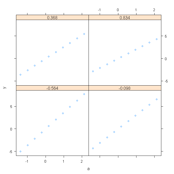
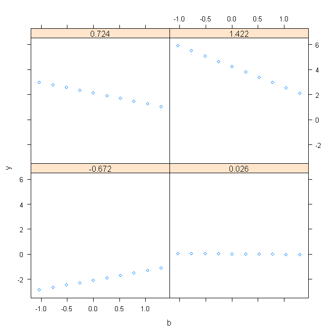
The two together don't tell you anything more than the second one would alone! The main effects are uninteresting and misleading when there is interaction present. The second model tells you all you need to know. Here are a couple of plots, with R code, to help you understand what that second model looks like...

library(lattice)

a <- rep(seq(-1.37, 2.12, (2.12--1.37)/9),4) 
b <- sort(rep(quantile(seq(-1.03, 1.30, .01),c(.2,.4,.6,.8)),10) )
y <- -0.06807 + (3.01517 * a) + (-0.00994 * b) + (-1.13782 *a*b)

xyplot(y~a|factor(b))

Effect of a on y by Levels of b

This one shows the estimated effect of a on y by levels of b. At each level of b, the relationship is positive. This is your significant positive slope for main effect of a in the presence of the interaction a:b.

a <- sort(rep(quantile(seq(-1.37, 2.12, .01),c(.2,.4,.6,.8)),10) )
b <- rep(seq(-1.03, 1.30, (1.30--1.03)/9),4) 
y <- -0.06807 + (3.01517 * a) + (-0.00994 * b) + (-1.13782 *a*b)

xyplot(y~b|factor(a))

Effect of b on y by Levels of a

This is image shows the estimated effects of b on y within levels of a. You can see why you have no significant main effect for b. The direction of the y~b relationship depends on level of a. Thus, no independent relationship (imagine averaging those lines) but a significant interaction (clear pattern when you take into account the level of a)

$\endgroup$
2
$\begingroup$

You may be interested by this introduction to the linear model (basis of almost any statistical analyses), and linear regression in particular:

  • it thoroughly explains lots of the mathematical aspects of linear regression, by detailing all important equations (which is usually left for exercise anywhere else on the Internet);
  • it uses a simple, yet informative enough, data set as an example;
  • and it gives all the R commands required to do the computations step by step, as well as plot the results.
$\endgroup$
2
$\begingroup$

If you want a book specifically on this sort of regression - as opposed to data analysis in general - I recommend Regression Analysis by Example by Chatterjee and Price. Good, not technical, but it doesn't oversimplify.

$\endgroup$

Your Answer

By clicking “Post Your Answer”, you agree to our terms of service and acknowledge you have read our privacy policy.

Not the answer you're looking for? Browse other questions tagged or ask your own question.