9
$\begingroup$

I have a few hundred estimates of a parameter calculated from two different models and I would like to know if these parameters have different variances.

What is a straightforward test for comparing the variances of these parameters? (straightforward meaning, least assumptions).

$\endgroup$
8
  • $\begingroup$ Are you comparing variances (as asserted in the first line) or means (as indicated in the third line)? $\endgroup$
    – whuber
    Commented Mar 21, 2011 at 21:24
  • $\begingroup$ @whuber I had confused myself; I have clarified my question. $\endgroup$
    – Abe
    Commented Mar 21, 2011 at 21:28
  • $\begingroup$ @Abe It seems now you have reversed "means" and "variances" but there's still a contradiction! (Unless perhaps you want to compare the variances of the means.) What do you mean by "variable": the means or the underlying values on which they are based? $\endgroup$
    – whuber
    Commented Mar 21, 2011 at 21:31
  • $\begingroup$ @whuber sorry, is that better? $\endgroup$
    – Abe
    Commented Mar 21, 2011 at 21:33
  • $\begingroup$ @Abe The new title helps a lot. But just to be clear: are the sigma-squareds the variances of the means or of the underlying variables upon which the means are based? $\endgroup$
    – whuber
    Commented Mar 21, 2011 at 21:35

1 Answer 1

9
$\begingroup$

For comparing variances, Wilcox suggests a percentile bootstrap method. See chapter 5.5.1 of 'Introduction to Robust Estimation and Hypothesis Testing'. This is available as comvar2 from the wrs package in R.

edit: to find the amount of bootstrap differences to trim from each side for different values of $\alpha$, one would perform a Monte Carlo study, as suggested by Wilcox. I have a quick and dirty one here in Matlab (duck from thrown shoes):

randn('state',0);           %to make the results replicable.
alphas = [0.001,0.005,0.01,0.025,0.05,0.10,0.15,0.20,0.25,0.333];
nreps  = 4096;
nsizes = round(2.^ (4:0.5:9));
nboots = 599;
cutls  = nan(numel(nsizes),numel(alphas));

for ii=1:numel(nsizes)
    n = nsizes(ii);
    imbalance = nan(nreps,1);
    for jj=1:nreps
        x1 = randn(n,1);x2 = randn(n,1);
        %make bootstrap samples;
        x1b = x1(ceil(n * rand(n,nboots)));
        x2b = x2(ceil(n * rand(n,nboots)));
        %compute stdevs
        sig1 = std(x1b,1);sig2 = std(x2b,1);
        %compute difference in stdevs
        Dvar = (sig1.^2 - sig2.^2);
        %compute the minimum of {the # < 0} and {the # > 0}
        %in (1-alpha) of the cases you want this minimum to match
        %your l number; then let u = 599 - l + 1
        imbalance(jj,1) = min(sum(Dvar < 0),sum(Dvar > 0));
    end
    imbalance = sort(imbalance);
    cutls(ii,:) = interp1(linspace(0,1,numel(imbalance)),imbalance(:)',alphas,'nearest');
end
%plot them;
lh = loglog(nsizes(:),cutls + 1);
legend(lh,arrayfun(@(x)(sprintf('alpha = %g',x)),alphas,'UniformOutput',false))
ylabel('l + 1');
xlabel('sample size, n_m');

I get the rather unhelpful plot: enter image description here
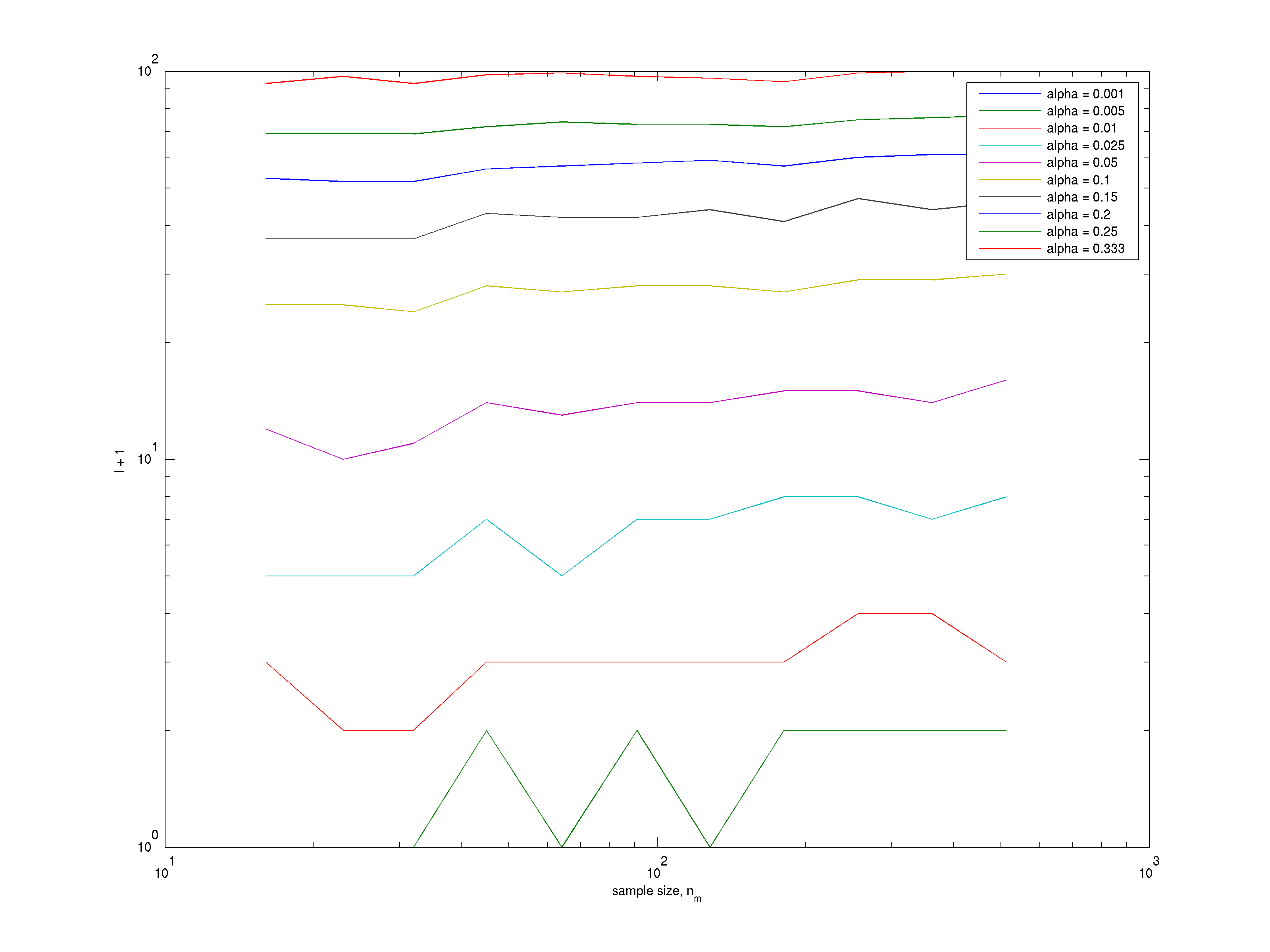
A little bit of hackery indicates that a model of the form $l + 0.5 = \exp{5.18} \alpha^{0.94} n^{0.067}$ fits my Monte Carlo simulations fairly well, but they do not give the same results that Wilcox quotes in his book. You might be better served running these experiments yourself at your preferred $\alpha$.

edit I ran this experiment again, using many more replicates ($2^{18}$) per sample size. Here's a table of the empirical values of $l$. The first row is a NaN, then the alpha (type I rate). Following that, the first column is the size of the samples, $n$, then the empirical values of $l$. (I would expect that as $n \to \infty$ we would have $l \to 599 \alpha /2$)

NaN,0.001,0.005,0.01,0.025,0.05,0.1,0.15,0.2,0.25,0.333
16,0,0,1,4,9,22,35,49,64,88
23,0,0,1,4,10,23,37,51,66,91
32,0,0,1,4,10,24,38,52,67,92
45,0,0,1,5,11,25,39,54,69,94
64,0,0,2,5,12,26,41,55,70,95
91,0,1,2,6,13,27,42,56,71,96
128,0,1,2,6,13,28,42,58,72,97
181,0,1,2,6,13,28,43,58,73,98
256,0,1,2,6,14,28,43,58,73,98
362,0,1,2,7,14,29,44,59,74,99
512,0,1,2,7,14,29,44,59,74,99
$\endgroup$
8
  • $\begingroup$ @shabbychef thanks for pointing me in this direction. It only took me about 5 min to download, read the section chapter, and compute; very much appreciated, but I am going to hold of on accepting your answer in hopes that other methods will be suggested - as this one is rather limited (only tests at alpha = 0.05, and there may be other options for large samples as in the present case) $\endgroup$
    – Abe
    Commented Mar 21, 2011 at 22:00
  • $\begingroup$ @shabbychef I've already +1 but was very unlucky with the R package -- OS X build doesn't include the aforementioned function :( $\endgroup$
    – chl
    Commented Mar 21, 2011 at 22:26
  • $\begingroup$ @chl AFAIK the package is just a convenient bundle for the functions that are available at www-rcf.usc.edu/~rwilcox/Rallfun-v13 $\endgroup$
    – caracal
    Commented Mar 21, 2011 at 22:42
  • $\begingroup$ @Abe: for values of $\alpha \ne 0.05$, Wilcox outlines the method for constructing the cutoff values of $l$ and $u$, but I agree it would be nice if they were available as rough functions of $\alpha$. $\endgroup$
    – shabbychef
    Commented Mar 21, 2011 at 22:46
  • $\begingroup$ @shabbychef I am confused - in the book it says 'the method can be applied only with $\alpha=0.05$, modifications based on other $\alpha$ values have not been derived"? His 2002 paper abstract hints otherwise, but I am not able to access it. $\endgroup$
    – Abe
    Commented Mar 21, 2011 at 22:50

Your Answer

By clicking “Post Your Answer”, you agree to our terms of service and acknowledge you have read our privacy policy.

Not the answer you're looking for? Browse other questions tagged or ask your own question.