As far as I know, when the variances are not equal, I can use Welch–Satterthwaite equation, my question is can I still use this equation although there is really a big difference between two samples? Or is there a certain limit for the difference between two samples?
The use of a scaled chi-square distribution with degrees of freedom from the Welch–Satterthwaite equation for the estimate of the variance of the difference in sample means is merely an approximation - the approximation is better under some circumstances than others.
In fact, I think any approach to this problem will be approximate in one way or another; this is the famous Behrens-Fisher problem. As it says at the upper right in the link there, only approximate solutions are known.
So the short answer is it's essentially never exactly correct -- and you can use it any time you like --- if you can tolerate the fact that your significance levels and p-values are inexact as a result; as for how far you can be out and still be happy to use it depends on you. Some people are much more tolerant of approximate significance levels and p-values than others*
*(in the situations that I tend to use hypothesis tests, as long as I know the direction and some sense of a bound on the extent of the effect, I tend to be pretty tolerant of significance levels different from nominal; but if I were trying to publish a scientific result in a journal, I'd probably document the likely impact of the approximation - via simulation - in more detail.)
So how does the approximation behave?
All distributions are normal:
The Welch test gives quite close to the right significance levels when the sample sizes are close to equal (on the other hand, the equal variance t-test also does fairly well when the sample sizes are equal, generally having only a moderate inflation of the significance level at smaller sample sizes).
Type I error rates become smaller than nominal ('conservative')
as the group sizes become more unequal. This affects both the Welch and the ordinary two sample test in the same direction. Power can also be low.
Distributions are skew:
If the distributions are skew, the effects on both significance level and power can be more substantial, and you must be much more wary (with skewness and unequal variances, I often lean toward using GLMs, as long as the variances seem likely to relate to the mean in an appropriate way - e.g. if spread increases with mean, a Gamma GLM may work well)
This document discusses a small simulation study of the Welch test, the ordinary t-test and a permutation test under equal and unequal variances, and normal distributions and a skewed distributions. It recommended:
the test with Welch correction is useful when the data are normal, sample sizes are small, and the variances are heterogeneous.
This seems broadly consistent with what I've read at other times.
However, in a later section, reading the details of the simulation results more deeply, they go on to say:
avoid the Welch-corrected t-test in the most extreme cases of sample size inequality (lower power)
Though that advice is based on very small sample sizes in the smaller sample. It was not carried out at the sort of sample sizes you have.
[When in doubt about the likely behavior of some procedure in some particular circumstance, I like run my own simulations. It's so easy in R that it's often a matter of only a couple of minutes - including coding, simulation runs and analysis of results - to get a good idea of the properties).]
I think that with one very large sample, and one medium sample size, as you have, there should still be relatively little problem applying Welch test. I'll double check with a simulation, right now.
My simulation results:
I used your sample sizes. These simulations are under normality.
First -- how badly is the test affected when $H_0$ is true?
a. The group with the large sample has 3 times the population standard deviation of the small one.
The Welch test achieves very close to the nominal type 1 error rate. The equal-variance t-test really doesn't; its significance levels are very very low, almost zero.
b. The group with the small sample has 3 times the population standard deviation of the large on.
The Welch test achieves very close to the nominal type 1 error rate. The equal-variance t-test doesn't; its significance levels are inflated.
In fact the equal-variance test was so badly affected, that I wouldn't use it at all; there would be little point in comparing power without adjusting for the difference in the significance levels.
With such a large sample size (meaning the uncertainty in its mean is relatively very small), another possibility presents itself: to do a one-sample test against the mean of the large sample as if it were fixed. It turns out that when the smaller population standard deviation was in the larger sample, significance levels were very close to nominal. It works relatively well in this case.
When the larger population standard deviation was in the larger sample, type 1 error rates were somewhat inflated (this looks to be the opposite direction from the effect on the Welch test).
A discussion of permutation tests
AdamO and I got into a discussion about an issue I have with permutation tests for this situation (different population variances in a test for location difference). He asked me for a simulation, so I'll do it here. The link to the paper I gave above also does simulations for the permutation test that seem to be broadly consistent with my findings.
The basic problem is in the two sample test of location with unequal variance, under the null the observations are not exchangeable. We cannot interchange labels without significantly affecting the results.
For example, imagine we had 334 observations where there was a 90% chance of having an $A$ label, and coming from a normal distribution with $\sigma=1$ and a 10% chance of having a $B$ label and coming from a normal distribution with $\sigma=3$. Further imagine that $\mu_A=\mu_B$. The observations are not exchangeable - in spite of most observations coming from sample $A$, the largest and smallest few observations are much more likely to have come from sample B than sample A and the middle observations are much more likely to have come from sample A (far more than the 90% chance they should have in the observations were exchangeable). This issue affects the distribution of p-values under the null. (However, if the sample sizes are equal, the effect is quite small.)
Let's see this with a simulation, as requested.
My code isn't especially fancy but it gets the job done. I simulate equal means for the sample sizes mentioned in the question, under three cases:
1) equal variance
2) the larger sample comes from a population with larger standard deviation (3 times as big as the other)
3) the smaller sample comes from a population with larger variance (3 times as big)
One of the things we're interested in with hypothesis tests is 'if I keep sampling these populations and do this test many times, what is my type I error rate'?
We can compute this here. The procedure consists of drawing normal samples fitting the above conditions, with the same mean, and then computing the quantile of the sample in the permutation distribution. Because we do this many times, this involves simulating many samples, and then within each sample, resampling many relabellings of the data to get the permutation distribution conditional on that sample. For every simulated sample I get a single p-value (by comparing the difference in means on the original sample with the permutation distribution for that specific sample). With many such samples, I get a distribution of p-values. This tell us the probability, given two populations with the same mean, we are to draw a sample where we reject the null (this is the Type I error rate).
Here's the code for one such simulation (case 2 above):
nperms <- 3000; nsamps <- 3000
n1 <- 310; n2 <- 34; ni12  <-  1/n1+1/n2
s1 <- 3; s2 <- 1

simpv  <-  function(n1,n2,s1,s2,nperms) {
  x <- rnorm(n1,s = s1);y <- rnorm(n2,s = s2)
  sdiff <- mean(x)-mean(y)
  xy <- c(x,y)
  sn1 <- sum(xy)/n1
  diffs <- replicate(nperms,sn1-sum(sample(xy,n2))*ni12)
  sum(sdiff<diffs)/nperms
}

pvs1big <- replicate(nsamps,simpv(n1,n2,s1,s2,nperms))
For the other two cases the code is the same, except I changed the s1= and s2= (and also changed what I stored the p-values in). For case 1, s1=1; s2=1 and for case 3 s1=1; s2=3
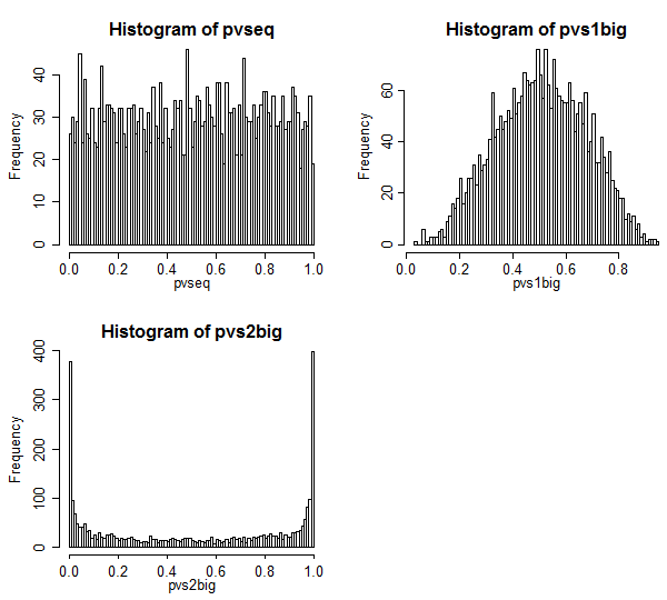
Now under the null, the distribution of p-values should be essentially uniform or we don't have the advertised type I error rate. (As performed the p-values are effectively for 1 tailed tests, but you can see what would happen for a two tailed test by looking at both ends of the distribution of p-values. They happen to be symmetric, so it doesn't matter.)
Here are the results.

Case 1 is at the top left. In this case the values are exchangeable, and we see a pretty uniform-looking distribution of p-values.
Case 2 is at the top right. In this case, the larger sample has the larger variance and we see that the p-values are concentrated toward the center. We are much less likely to reject a null case at typical significance levels than we think we should. That is, the type I error rate is much lower than the nominal rate.
Case 3 is at the bottom right. In this case, the smaller sample has the larger variance, and we see that the p-values are concentrated at the two ends - under the null, we are much more likely to reject than we think we should. The significance level is much higher than the nominal rate.
Discussion of the Behrens Fisher problem in Good
The Good Book mentioned by AdamO does discuss this problem on p54-57.
He refers to a result of Romano that states that the permutation test is asymptotically exact providing they have equal sample sizes. Here, of course, they don't - rather than 50-50 they're roughly 90-10.
And when I simulate the equal sample size case (I tried n1=n2=34) the p-value distribution wasn't far off uniform** -- it was off a small amount but not enough to worry about. This is pretty well known and borne out by a number of published simulation studies.
**(I haven't included the code, but it's trivial to adapt the above code to do it - just change n1 to be 34)
Good says the behavior in the equal sample size case works down to quite small sample sizes. I believe him!
What about a bootstrap test?
So what if we were to try a bootstrap test instead of a permutation test?
With a bootstrap test*, my objections no longer hold.
*e.g. one approach might be to construct a CI for the difference in means and reject at the 5% level if a 95% interval for the mean doesn't include 0
With a bootstrap test, we're no longer required to be able to relabel across samples -- we can resample within the samples we have and still get a suitable CI for the difference in means. With some of the usual procedures to improve the properties of the bootstrap, such a test might work very well at these sample sizes.

