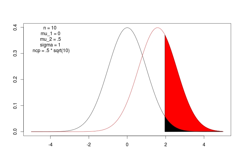
In power calculations, we calibrate tests using knowledge of what the sampling distribution of the test statistic would be under the null hypothesis. Usually, it follows a $\chi^2$ or normal distribution. This allows you to calculate "critical values" for which, values exceeding this are deemed to be too highly inconsistent with what would be expected if the null were true.
The power of a statistical test is calculated by specifying the probability model for the data generating process under an alternative hypothesis, and calculating the sampling distribution for the same test statistic. This now takes on a different distribution.
For test statistics having a $\chi^2$ distribution under the null, they take a non-central $\chi^2$ distribution under the alternative that you create. These are very complicated distributions, but standard software can calculate density, distribution, and quantiles for them easily. The trick is that they are a convolution of standard $\chi^2$ densities and Poisson densities. In R, the dchisq, pchisq, and rchisq functions all have an optional ncp argument which is, by default, 0.
If the test statistic has a standard normal distribution under the null hypothesis, it will have a nonzero mean normal distribution under the alternative. Here that mean is the noncentrality parameter. For a t-test under an equal variance assumption, the mean is given by:
$$\delta = \frac{\mu_1 -\mu_2}{\sigma_{pooled}/\sqrt{n}}$$

In either case, data generated according to an alternative hypothesis will have test statistics following some noncentral distribution with noncentrality parameter ($\delta$). The $\delta$ is a sometimes unknown, often complicated function of the other data generating parameters.

