How is sample mean divided by sample STD distributed for normal distributions?

Question

Let's assume that we sample N times from a normal distribution with known mean and variance. With a generated sample we calculate sample mean and sample standard deviation. Then we divide sample mean by sample standard deviation (STD) to get the measure of my interest.

The question that I have: Is there an analytical expression for the distribution of the above described measure?

I know that distribution for the sample mean is well known. I have also found an expression for the distribution of sample STD. However, I cannot find the distribution that I need.

Answer 1

Let $X_1,...,X_n \sim \text{IID N}(\mu, \sigma)$ be your data points. It is well known from Cochran's theorem that the sample mean and sample variance are independent with distributions:

$$\bar{X}_n \sim \text{N} \Big( \mu, \frac{\sigma^2}{n} \Big) \quad \quad \quad S_n^2 \sim \sigma^2 \cdot \frac{\text{Chi-Sq}(n-1)}{n-1}.$$

Hence, we can form the independent statistics:

$$Z_n \equiv \frac{\bar{X}_n - \mu}{\sigma / \sqrt{n}} \sim \text{N}(0,1) \quad \quad \quad \chi_n \equiv \frac{S_n}{\sigma} \sim \frac{\text{Chi}(n-1)}{\sqrt{n-1}}.$$

With a bit of algebra we then have:

$$\begin{equation} \begin{aligned} \frac{\bar{X}_n}{S_n} &= \frac{\bar{X}_n / \sigma}{S_n / \sigma} \\[6pt] &= \frac{\bar{X}_n / \sigma}{\chi_n} \\[6pt] &= \frac{1}{\sqrt{n}} \cdot \frac{\sqrt{n} \bar{X}_n / \sigma}{\chi_n} \\[6pt] &= \frac{1}{\sqrt{n}} \cdot \frac{\sqrt{n} (\bar{X}_n - \mu)/\sigma + \sqrt{n} \mu/\sigma}{\chi_n} \\[6pt] &= \frac{1}{\sqrt{n}} \cdot \frac{Z_n + \sqrt{n} \mu/\sigma}{\chi_n} \\[6pt] &\sim \frac{1}{\sqrt{n}} \cdot \text{Noncentral T} \big(\sqrt{n} \mu/\sigma, n-1 \big). \\[6pt] \end{aligned} \end{equation}$$

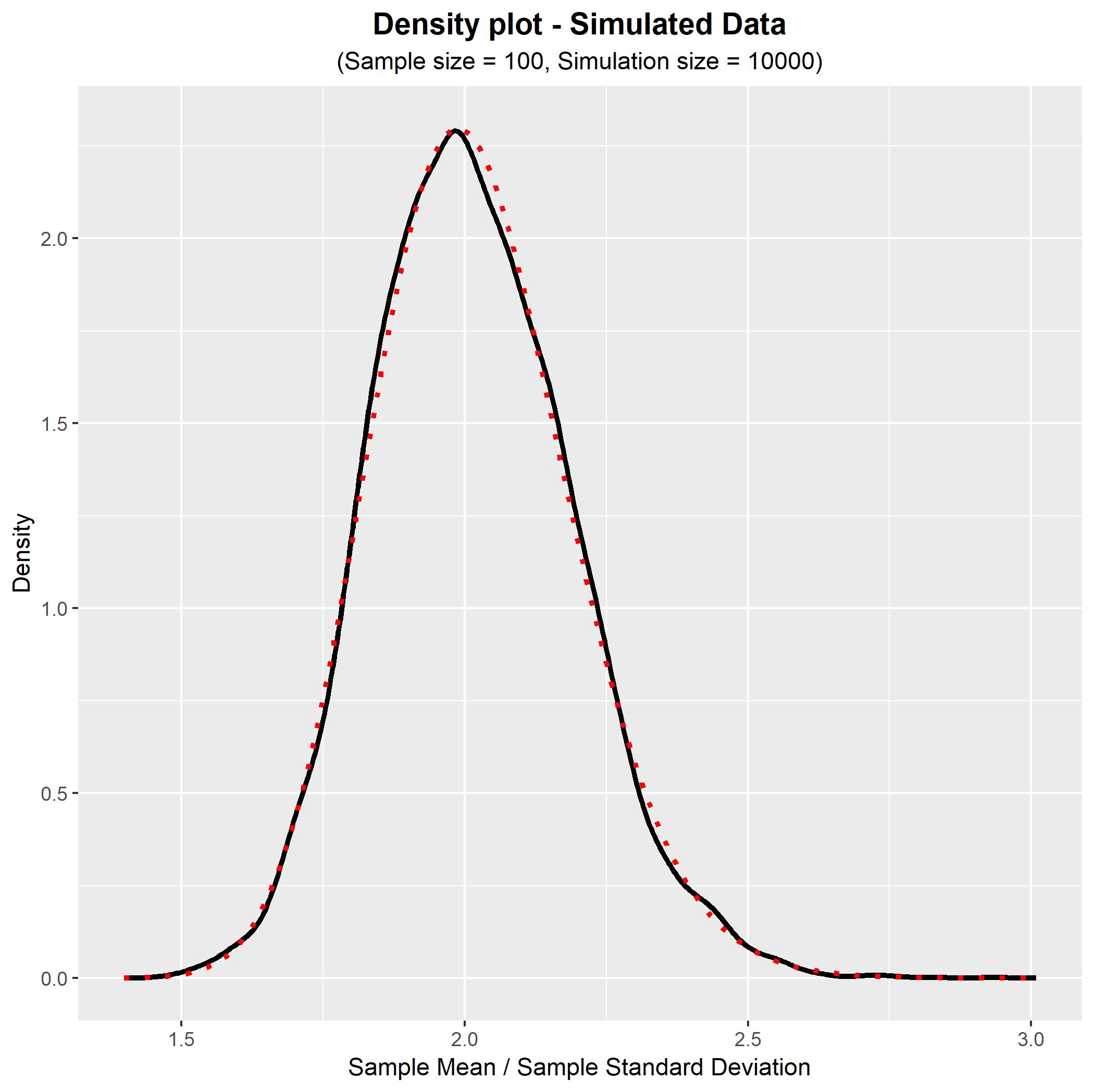
So you can see that the ratio of the sample mean on the sample standard deviation has a scaled non-central T distribution with non-centrality parameter $\sqrt{n} \mu/\sigma$ and degrees-of-freedom $n-1$. We can double-check this theoretical result empirically via simulation.

---

Checking the distribution by simulation: In the R code below we create a function to simulate $m$ samples of size $n$ from the IID normal model and generate the $m$ ratio statistics from these samples. We plot the kernel density of these simulated statistics against the theoretical distribution above in order to confirm that the theoretical result is correct.

#Simulate m values of the ratio statistic for samples of size n
SIMULATE <- function(m, n, mu, sigma) { 
              X <- array(rnorm(n*m, mean = mu, sd = sigma), dim = c(m,n));
              R <- rep(0, m);
              for (i in 1:m) { R[i] <- mean(X[i,])/sd(X[i,]); }
              R; }

#Plot the density of the simulated values against theoretical
PLOTSIM  <- function(m, n, mu, sigma) { 
              require(stats); require(ggplot2);
              RR    <- SIMULATE(m, n, mu, sigma);
              DENS  <- density(RR);
              DENS$yy <- dt(DENS$x*sqrt(n), df = n-1, ncp = sqrt(n)*mu/sigma)*sqrt(n);
              DATA <- data.frame(x = DENS$x, y = DENS$y, yy = DENS$yy);
              ggplot(data = DATA, aes(x = x)) +
                geom_line(aes(y = y), size = 1.2, colour = 'black') +
                geom_line(aes(y = yy), size = 1.2, colour = 'red', linetype = 'dotted') +
                theme(plot.title    = element_text(hjust = 0.5, size = 14, face = 'bold'),
                      plot.subtitle = element_text(hjust = 0.5)) +
                ggtitle('Density plot - Simulated Data') +
                labs(subtitle = 
                     paste0('(Sample size = ', n, ', Simulation size = ', m, ')')) +
                xlab('Sample Mean / Sample Standard Deviation') +
                ylab('Density'); }

#Generate example plot
set.seed(1);
m     <- 10^4;
n     <- 100;
mu    <- 12;
sigma <- 6;

PLOTSIM(m, n, mu, sigma);

Answer 2

@Roman, here is my Python code, of @Ben's example above

• it produces a file "walks.tsv" with N realisations of a random walk with mean=μ and stdev=σ.

• for each realisation there is a row, with the sample mean, sample stdev, and sample mean/stdev.

• I loaded "walk.tsv" in Excel and used Excel to aggregate and plot the data.

Hope it helps 🙂

import math, numpy.random

class RandomWalk:

    def __init__(self, step_mean, step_stdev, steps_per_walk):
        self.step_mean = step_mean
        self.step_stdev = step_stdev
        self.steps = steps_per_walk
        self.log = open("walk.tsv","w+")
        self.log_names()

    def realize(self):
        total = 0
        total_sqr = 0
        for i in range(self.steps):
            step = float(numpy.random.normal(self.step_mean, self.step_stdev, 1))
            total += step
            total_sqr += step * step
        self.sample_mean = total / self.steps
        self.sample_stdev = math.sqrt(total_sqr / self.steps - self.sample_mean * self.sample_mean)
        self.log_values()

    def log_names(self):
        self.log.write("dist_mean\t")
        self.log.write("dist_stdev\t")
        self.log.write("dist_mean/stdev\t")
        self.log.write("steps\t")
        self.log.write("sample_mean\t")
        self.log.write("sample_stdev\t")
        self.log.write("sample_mean/stdev\n")
        self.log.flush()

    def log_values(self):
        self.log.write("{:0.1f}\t".format(self.step_mean))
        self.log.write("{:0.1f}\t".format(self.step_stdev))
        self.log.write("{:0.2f}\t".format(self.step_mean / self.step_stdev))
        self.log.write("{}\t".format(self.steps))
        self.log.write("{:0.1f}\t".format(self.sample_mean))
        self.log.write("{:0.1f}\t".format(self.sample_stdev))
        self.log.write("{:0.2f}\n".format(self.sample_mean / self.sample_stdev))
        self.log.flush()


def simulate(step_mean, step_stdev, steps_per_walk, walks):
    walk = RandomWalk(step_mean, step_stdev, steps_per_walk)
    for i in range(walks):
        walk.realize()

simulate(step_mean = 12, step_stdev = 6, steps_per_walk = 100, walks = 10000)