How large does the sample size need for the t distribution to be approximately normal

Question

According to my understanding, when we have unknown population mean and variance, we have to estimate population variance through sample variance and use the t distribution to estimate the potential range of the population mean using the estimated population variance and sample mean under a certain level of confidence. The t distribution has a heavier tail when degrees of freedom are few because we are using estimated population variance, not the true population variance, which includes a certain degree of uncertainty. When sample size = 30, the t distribution will be closer to the z distribution, as the estimated population variance is close to the true population variance(?).

I recently run a simulation with a sample of $n = 30$ and repeated that 1000 times. I calculated the mean of the unbiased sample variance, and it is close to the population variance (normal distributed population). However, the variance (SD) of sample variance is still huge. SD of variance / variance = 20 to 30%. That means if we are unlucky, we may get a sample with sample variance much larger or smaller than the true population variance. Why then will the t distribution look so similar to the z distribution when the uncertainty of the population variance is still so huge for $n = 30$?

I always thought that we use the t distribution instead of z because it somehow helps us to involve the uncertainty of the estimated population variance in the equation. Why does this effect / compensation go away when $n=30$? The distribution of sample variance is still widely spread when $n = 30$. Could anyone please explain to me? Thanks a lot!

Answer 1

If you knew the true standard deviation, then the parameter estimate over its dispersion would have been from z, the standard normal distribution: $z=\hat{\beta}/\sigma\sim\mathcal{N}(0,1)$, Rarely you know it, so the t-statistics $t=\hat{\beta}/\hat{\sigma}\sim\mathcal{t}(d.f.)$

Since $t_\infty=\mathcal{N}(0,1)$ in statistical tables at high enough degrees of freedom the standard normal distribution is used. Frankly, I never seen a table where "high enough" was 30. It usually is higher than 100 or 200.

I know of one rule of thumb with 30, which is the number of random variable in a sum to apply CLT to a sum. This number was suggested in a work to which I lost the reference, unfortunately.

Answer 2

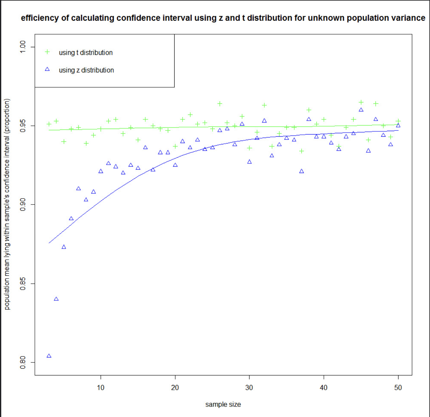
thank you for everyone comments and answers. i have run another simulation using sample = n (from 3 to 50), repeating 1000 times and plot the result here (the population is also normal distribution). I think i can now understand why z distribution can replace t distribution when sample size get large.

is.between <- function(x, a, b) {
  x > a & x < b
}
set.seed(09101165)
population<-rnorm(n=10000, mean=100, sd =10)
##population<-runif(n=10000, min=50,max=100)
## you can use runif() instead of rnorm for generating a evenly distributed population
mean_of_population<-mean(population)
var(population)
## var = 102.5493
master_of_sample<-list()
for (ss in 3:50){
  group_of_sample<-list()
  for (i in 1:1000){
    group_of_sample[[i]]<-sample(population,size=ss)
  }
  master_of_sample[[ss]]<-group_of_sample
}
Mean<-vector()
Variance<-vector()
upper_interval<-vector()
lower_interval<-vector()
upper_interval2<-vector()
lower_interval2<-vector()
within_confidence_interval<-logical()
within_confidence_interval2<-logical()
finalt<-vector()
finalz<-vector()

for (ss in 3:50){
  Mean<-vector()
  Variance<-vector()
  upper_interval<-vector()
  lower_interval<-vector()
  within_confidence_interval<-logical()
  for (i in 1:1000){Mean[i]<-mean(master_of_sample[[ss]][[i]])
                    Variance[i]<-var(master_of_sample[[ss]][[i]])
                    upper_interval[i]<-Mean[i]+qt(0.975,df=(ss-1))*(sqrt(Variance[i]/ss))
                    lower_interval[i]<-Mean[i]-qt(0.975,df=(ss-1))*(sqrt(Variance[i]/ss))
                    upper_interval2[i]<-Mean[i]+qnorm(0.975)*(sqrt(Variance[i]/ss))
                    lower_interval2[i]<-Mean[i]-qnorm(0.975)*(sqrt(Variance[i]/ss))
                    within_confidence_interval[i]<-is.between(mean_of_population,lower_interval[i],upper_interval[i])
                    within_confidence_interval2[i]<-is.between(mean_of_population,lower_interval2[i],upper_interval2[i])
 }
  finalt[ss]<-sum(within_confidence_interval)/length(within_confidence_interval)
  finalz[ss]<-sum(within_confidence_interval2)/length(within_confidence_interval2)
}

plot(y=finalt[3:50], x=3:50,ylim=c(0.8,1),type="n", ylab="population mean lying within sample's confidence interval (proportion)", xlab="sample size", 
     main="efficiency of calculating confidence interval using z and t distribution for unknown population variance" )
points(y=finalt[3:50], x=3:50,col="green",pch=3)
fort<-smooth.spline(finalt[3:50]~3:50,df=3)
lines(fort,col="green")
points(y=finalz[3:50], x=3:50,col="blue",pch=2 )
forz<-smooth.spline(finalz[3:50]~3:50,df=3)
lines(forz,col="blue")
legend("topleft",legend=c("using t distribution","using z distribution"),pch=c(3,2),col=c("green","blue"))